This vignette1 discusses in-sample and out-of-sample prediction within RprobitB. The former case refers to reproducing the observed choices on the basis of the covariates and the fitted model and subsequently using the deviations between prediction and reality as an indicator for the model performance. The latter means forecasting choice behavior for changes in the choice attributes.
For illustration, we revisit the probit model of travelers deciding between two fictional train route alternatives from the vignette on model fitting:
form <- choice ~ price + time + change + comfort | 0
data <- prepare_data(form = form, choice_data = train_choice, id = "deciderID", idc = "occasionID")
model_train <- fit_model(
  data = data,
  scale = "price := -1"
)
Reproducing the observed choices
RprobitB provides a predict() method for
RprobitB_fit objects. Per default, the method returns a
confusion matrix, which gives an overview of the in-sample prediction
performance:
predict(model_train)
#>     predicted
#> true    A    B
#>    A 1030  444
#>    B  447 1008
By setting the argument overview = FALSE, the method
instead returns predictions on the level of individual choice
occasions:
pred <- predict(model_train, overview = FALSE)
head(pred, n = 10)
#>    deciderID occasionID    A    B true predicted correct
#> 1          1          1 0.92 0.08    A         A    TRUE
#> 2          1          2 0.64 0.36    A         A    TRUE
#> 3          1          3 0.79 0.21    A         A    TRUE
#> 4          1          4 0.18 0.82    B         B    TRUE
#> 5          1          5 0.55 0.45    B         A   FALSE
#> 6          1          6 0.13 0.87    B         B    TRUE
#> 7          1          7 0.55 0.45    B         A   FALSE
#> 8          1          8 0.76 0.24    B         A   FALSE
#> 9          1          9 0.55 0.45    A         A    TRUE
#> 10         1         10 0.60 0.40    A         A    TRUE
Among the three incorrect predictions shown here, the one for decider
id = 1 in choice occasion idc = 8 is the most
outstanding. Alternative B was chosen although the model
predicts a probability of 75% for alternative A. We can use
the convenience function get_cov() to extract the
characteristics of this particular choice situation:
get_cov(model_train, id = 1, idc = 8)
#>   deciderID occasionID choice  price_A   time_A change_A comfort_A  price_B
#> 8         1          8      B 52.88904 1.916667        0         1 70.51872
#>   time_B change_B comfort_B
#> 8    2.5        0         0
The trip option A was 20€ cheaper and 30 minutes faster,
which by our model outweighs the better comfort class for alternative
B, recall the estimated effects:
coef(model_train)
#>            Estimate   (sd)
#> 1   price     -1.00 (0.00)
#> 2    time    -25.15 (1.98)
#> 3  change     -4.81 (0.86)
#> 4 comfort    -14.29 (0.87)
The misclassification can be explained by preferences that differ from the average decider (choice behavior heterogeneity), or by unobserved factors that influenced the choice. Indeed, the variance of the error term was estimated high:
point_estimates(model_train)$Sigma
#>          [,1]
#> [1,] 651.0734
#> attr(,"names")
#> [1] "1,1"
Apart from the prediction accuracy, the model performance can be
evaluated more nuanced in terms of sensitivity and specificity. The
following snippet exemplary shows how to visualize these measures by
means of a receiver operating characteristic (ROC) curve (Fawcett 2006), using the
plotROC package (Sachs 2017). The
curve is constructed by plotting the true positive fraction against the
false positive fraction at various cutoffs (here
n.cuts = 20). The closer the curve is to the top-left
corner, the better the binary classification.
library(plotROC)
ggplot(data = pred, aes(m = A, d = ifelse(true == "A", 1, 0))) +
  geom_roc(n.cuts = 20, labels = FALSE) +
  style_roc(theme = theme_grey)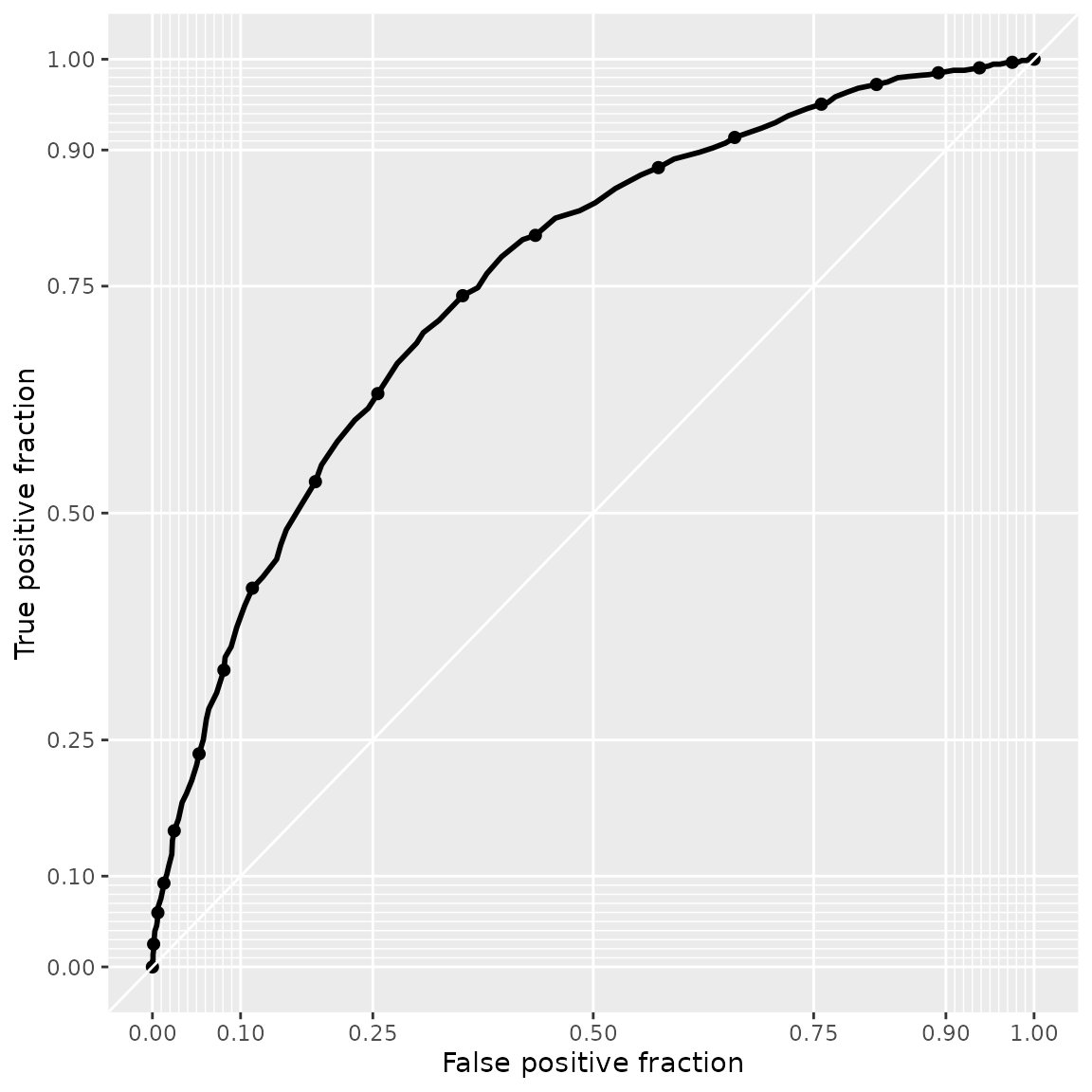
Forecasting choice behavior
The predict() method has an additional data
argument. Per default, data = NULL, which results into the
in-sample case outlined above. Alternatively, data can be
either
an
RprobitB_dataobject (for example the test subsample derived from thetrain_test()function, see the vignette on choice data),or a data frame of custom choice characteristics.
We demonstrate the second case in the following. Assume that a train company wants to anticipate the effect of a price increase on their market share. By our model, increasing the ticket price from 100€ to 110€ (ceteris paribus) draws 15% of the customers to the competitor who does not increase their prices.
predict(
  model_train,
  data = data.frame(
    "price_A" = c(100, 110),
    "price_B" = c(100, 100)
  ),
  overview = FALSE
)
#>   deciderID occasionID    A    B prediction
#> 1         1          1 0.50 0.50          A
#> 2         2          1 0.35 0.65          B
However, offering a better comfort class compensates for the higher price and even results in a gain of 7% market share: