The goal of RprobitB is to explain choices made by deciders among a discrete set of alternatives. In a Bayesian way. For example, think of tourists that want to book a train trip to their holiday destination: The knowledge why they prefer a certain alternative over another is of great value for train companies, especially the customer’s willingness to pay for say a faster or more comfortable trip.
Installation
You can install the released version of RprobitB from CRAN with:
install.packages("RprobitB")Documentation
The package is documented in several vignettes, see here.
Example
We analyze a data set of 2929 stated choices by 235 Dutch individuals deciding between two virtual train trip options based on the price, the travel time, the level of comfort, and the number of changes.
library("RprobitB")
#> Thanks for using {RprobitB} version 1.1.3, happy choice modeling!
#> Documentation: https://loelschlaeger.de/RprobitB
The following lines fit a probit model that explains the chosen trip alternatives (choice) by their price, time, number of changes, and level of comfort (the lower this value the higher the comfort). For normalization, the first linear coefficient, the price, is fixed to -1, which allows to interpret the other coefficients as monetary values:
form <- choice ~ price + time + change + comfort | 0
data <- prepare_data(form, train_choice, id = "deciderID", idc = "occasionID")
model <- fit_model(data, scale = "price := -1")
The estimated effects can be visualized via:
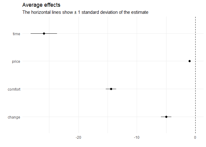
The results indicate that the deciders value one hour travel time by about 25€, an additional change by 5€, and a more comfortable class by 15€.
Now assume that a train company wants to anticipate the effect of a price increase on their market share. By our model, increasing the ticket price from 100€ to 110€ (ceteris paribus) draws 15% of the customers to the competitor who does not increase their prices:
predict(
  model,
  data = data.frame(
    "price_A" = c(100, 110),
    "price_B" = c(100, 100)
  ),
  overview = FALSE
)
#> Checking for missing covariates
#>   deciderID occasionID    A    B prediction
#> 1         1          1 0.50 0.50          A
#> 2         2          1 0.35 0.65          B
However, offering a better comfort class (0 here is better than 1) compensates for the higher price and even results in a gain of 7% market share: