Alternating optimization • ao

The ao package implements alternating optimization in R. This vignette demonstrates the main workflow and describes the available customization options.

What is alternating optimization?

Alternating optimization (AO) is an iterative process for optimizing a multivariate function by breaking it into simpler sub-problems. In each step, AO optimizes over one block of parameters while keeping the other blocks fixed, then alternates among the blocks. AO is particularly useful when the sub-problems are easier to solve than the original joint optimization problem, or when the parameters have a natural partition. See Bezdek and Hathaway (2002), Hu and Hathaway (2002), and Bezdek and Hathaway (2003) for more details.

Consider a real-valued objective function $f(\mathbf{x}, \mathbf{y})$ where $\mathbf{x}$ and $\mathbf{y}$ are two blocks of function parameters, namely a partition of the parameters. The AO process can be described as follows:

Initialization: Start with initial guesses $\mathbf{x}^{(0)}$ and $\mathbf{y}^{(0)}$ .
Iterative Steps: For $k = 0, 1, 2, \dots$
- Step 1: Fix $\mathbf{y} = \mathbf{y}^{(k)}$ and solve the sub-problem $\mathbf{x}^{(k+1)} = \arg \min_{\mathbf{x}} f(\mathbf{x}, \mathbf{y}^{(k)}).$
- Step 2: Fix $\mathbf{x} = \mathbf{x}^{(k+1)}$ and solve the sub-problem $\mathbf{y}^{(k+1)} = \arg \min_{\mathbf{y}} f(\mathbf{x}^{(k+1)}, \mathbf{y}).$
Convergence: Repeat the iterative steps until a convergence criterion is met, such as when the change in the objective function or the parameters falls below a specified threshold, or when a predefined iteration limit is reached.

The AO process can be

viewed as a generalization of joint optimization, where the parameter partition is trivial, consisting of the entire parameter vector as a single block,
also used for maximization problems by simply replacing $\arg \min$ by $\arg \max$ above,
generalized to more than two parameter blocks, i.e., for $f(\mathbf{x}_1, \mathbf{x}_2, \ldots, \mathbf{x}_n)$ , the process involves cycling through each parameter block $\mathbf{x}_1, \mathbf{x}_2, \ldots, \mathbf{x}_n$ and solving the corresponding sub-problems iteratively (the parameter blocks do not necessarily have to be disjoint),
randomized by changing the parameter partition randomly after each iteration, which can further improve the convergence rate and help avoid getting trapped in local optima (Chib and Ramamurthy 2010),
run in multiple processes for different initial values, parameter partitions, and/or base optimizers.

How to use the package?

The ao package provides one user-level function, ao(), as the general interface for different AO variants.

The function call

The ao() function call with the default arguments looks as follows:

ao(
  f,
  initial,
  target = NULL,
  npar = NULL,
  gradient = NULL,
  hessian = NULL,
  ...,
  partition = "sequential",
  new_block_probability = 0.3,
  minimum_block_number = 1,
  minimize = TRUE,
  lower = NULL,
  upper = NULL,
  iteration_limit = Inf,
  seconds_limit = Inf,
  tolerance_value = 1e-6,
  tolerance_parameter = 1e-6,
  tolerance_parameter_norm = function(x, y) sqrt(sum((x - y)^2)),
  tolerance_history = 1,
  base_optimizer = optimizeR::Optimizer$new(
    "stats::optim", method = "L-BFGS-B"
  ),
  verbose = FALSE,
  hide_warnings = TRUE,
  add_details = TRUE
)

The arguments have the following meaning:

f: The objective function to be optimized. By default, f is optimized over its first argument. If optimization should target a different argument or multiple arguments, use npar and target, see below. Additional arguments for f can be passed via the ... argument as usual.
initial: Initial values for the parameters used in the AO process.
gradient and hessian: Optional arguments to specify the analytic gradient and/or Hessian of f.
partition: Specifies how parameters are partitioned for optimization. Can be one of the following:
- "sequential": Optimizes each parameter block sequentially. This is similar to coordinate descent.
- "random": Randomly partitions parameters in each iteration.
- "none": No partitioning; equivalent to joint optimization.
- Custom partition can be defined using a list of vectors of parameter indices, see below.
new_block_probability and minimum_block_number are only relevant if partition = "random". In this case, the former controls the probability for creating a new block when building a random parameter partition, and the latter defines the minimum number of parameter blocks in the partition.
minimize: Set to TRUE for minimization (default), or FALSE for maximization.
lower and upper: Lower and upper limits for constrained optimization.
iteration_limit is the maximum number of AO iterations before termination, while seconds_limit is the time limit in seconds. tolerance_value and tolerance_parameter (in combination with tolerance_parameter_norm) specify two other stopping criteria: the current function value or parameter vector must differ from its value tolerance_history iterations earlier by less than the corresponding threshold.
base_optimizer: Numerical optimizer used for solving sub-problems, see below.
Set verbose to TRUE to print status messages, and hide_warnings to FALSE to show warnings during the AO process. add_details = TRUE adds process details to the output.

A simple first example

The following is an implementation of the Himmelblau’s function $f(x, y) = (x^2 + y - 11)^2 + (x + y^2 - 7)^2:$

himmelblau <- function(x) (x[1]^2 + x[2] - 11)^2 + (x[1] + x[2]^2 - 7)^2

This function has four identical local minima, for example in $x = 3$ and $y = 2$ :

himmelblau(c(3, 2))
#> [1] 0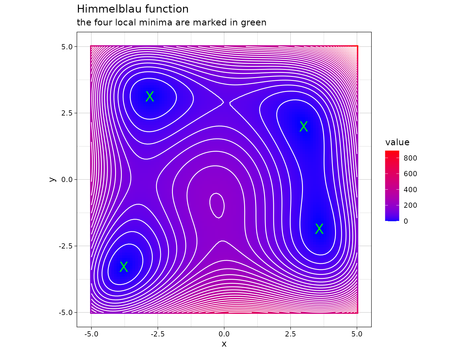

Minimizing Himmelblau’s function through alternating minimization over $\mathbf{x}$ and $\mathbf{y}$ with initial values $\mathbf{x}^{(0)} = \mathbf{y}^{(0)} = 0$ can be accomplished as follows:

ao(f = himmelblau, initial = c(0, 0))
#> $estimate
#> [1]  3.584428 -1.848126
#> 
#> $value
#> [1] 9.606386e-12
#> 
#> $details
#>    iteration        value       p1        p2 b1 b2     seconds
#> 1          0 1.700000e+02 0.000000  0.000000  0  0 0.000000000
#> 2          1 1.327270e+01 3.395691  0.000000  1  0 0.041499138
#> 3          1 1.743664e+00 3.395691 -1.803183  0  1 0.009001493
#> 4          2 2.847290e-02 3.581412 -1.803183  1  0 0.006982088
#> 5          2 4.687468e-04 3.581412 -1.847412  0  1 0.006034851
#> 6          3 7.368057e-06 3.584381 -1.847412  1  0 0.005048513
#> 7          3 1.164202e-07 3.584381 -1.848115  0  1 0.049827576
#> 8          4 1.893311e-09 3.584427 -1.848115  1  0 0.004145384
#> 9          4 9.153860e-11 3.584427 -1.848124  0  1 0.003338099
#> 10         5 6.347425e-11 3.584428 -1.848124  1  0 0.003342152
#> 11         5 9.606386e-12 3.584428 -1.848126  0  1 0.003147602
#> 
#> $seconds
#> [1] 0.1323669
#> 
#> $stopping_reason
#> [1] "change in function value between 1 iteration is < 1e-06"

Here, we see the output of the AO process, which is a list that contains the following elements:

estimate is the parameter vector at termination.
value is the function value at termination.
details is a data.frame with full information about the process: For each iteration (column iteration) it contains the function value (column value), parameter values (columns starting with p followed by the parameter index), the active parameter block (columns starting with b followed by the parameter index, where 1 stands for a parameter contained in the active parameter block and 0 if not), and computation times in seconds (column seconds).
seconds is the overall computation time in seconds.
stopping_reason is a message explaining why the process terminated.

Using the analytic gradient

For Himmelblau’s function, the analytic gradient is:

gradient <- function(x) {
  c(
    4 * x[1] * (x[1]^2 + x[2] - 11) + 2 * (x[1] + x[2]^2 - 7),
    2 * (x[1]^2 + x[2] - 11) + 4 * x[2] * (x[1] + x[2]^2 - 7)
  )
}

The gradient function is used by ao() if provided via the gradient argument as follows:

ao(f = himmelblau, initial = c(0, 0), gradient = gradient, add_details = FALSE)
#> $estimate
#> [1]  3.584428 -1.848126
#> 
#> $value
#> [1] 2.659691e-12
#> 
#> $seconds
#> [1] 0.05126333
#> 
#> $stopping_reason
#> [1] "change in function value between 1 iteration is < 1e-06"

In higher-dimensional problems, using the analytic gradient can improve both the speed and stability of the process. An analytic Hessian can be supplied in the same way.

Random parameter partitions

Another AO variant uses a new random partition of the parameters in every iteration. This can improve convergence and help prevent the process from getting stuck in local optima. It is activated by setting partition = "random". The randomness can be adjusted using two parameters:

new_block_probability determines the probability of creating a new block when building a new partition. Its value ranges from 0 (no blocks are created) to 1 (each parameter is a single block).
minimum_block_number sets the minimum number of parameter blocks for random partitions. Here, it is configured as 2 to avoid generating trivial partitions.

Random partitions are generated as follows:¹

process <- ao:::Process$new(
  npar = 10,
  partition = "random",
  new_block_probability = 0.5,
  minimum_block_number = 2
)
process$get_partition()
#> [[1]]
#> [1] 5
#> 
#> [[2]]
#> [1] 1 6 9
#> 
#> [[3]]
#> [1] 10
#> 
#> [[4]]
#> [1] 7
#> 
#> [[5]]
#> [1] 4 8
#> 
#> [[6]]
#> [1] 2 3
process$get_partition()
#> [[1]]
#> [1] 1 7 8
#> 
#> [[2]]
#> [1]  6 10
#> 
#> [[3]]
#> [1] 3 4
#> 
#> [[4]]
#> [1] 2
#> 
#> [[5]]
#> [1] 9
#> 
#> [[6]]
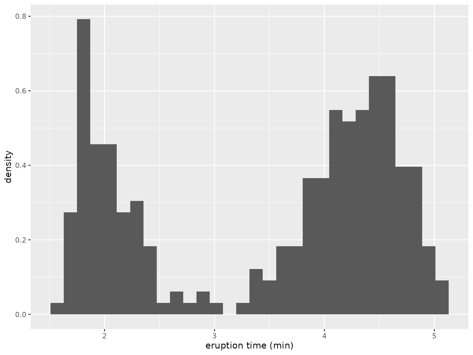
#> [1] 5

As an example of AO with random partitions, consider fitting a two-class Gaussian mixture model via maximizing the model’s log-likelihood function

$\ell(\boldsymbol{\theta}) = \sum_{i=1}^n \log\Big( \lambda \phi_{\mu_1, \sigma_1^2}(x_i) + (1-\lambda)\phi_{\mu_2,\sigma_2^2} (x_i) \Big),$

where the sum is over all observations $x_1, \dots, x_n$ , $\phi_{\mu_1, \sigma_1^2}$ and $\phi_{\mu_2, \sigma_2^2}$ denote the normal density for the first and second cluster, respectively, and $\lambda$ is the mixing proportion. The parameter vector to be estimated is $\boldsymbol{\theta} = (\mu_1, \mu_2, \sigma_1, \sigma_2, \lambda)$ . Because there is no closed-form solution for the maximum likelihood estimator $\boldsymbol{\theta}^* = \arg\max_{\boldsymbol{\theta}} \ell(\boldsymbol{\theta})$ , we use numerical optimization to find the optimum. The model is fitted to the following data:²

The following function calculates the log-likelihood value given the parameter vector theta and the observation vector data:³

normal_mixture_llk <- function(theta, data) {
  mu <- theta[1:2]
  sd <- exp(theta[3:4])
  lambda <- plogis(theta[5])
  c1 <- lambda * dnorm(data, mu[1], sd[1])
  c2 <- (1 - lambda) * dnorm(data, mu[2], sd[2])
  sum(log(c1 + c2))
}

The ao() call for performing alternating maximization with random partitions looks as follows, where we simplified the output for brevity:

out <- ao(
  f = normal_mixture_llk,
  initial = runif(5),
  data = datasets::faithful$eruptions,
  partition = "random",
  minimize = FALSE
)
round(out$details, 2)
#>    iteration   value   p1   p2    p3    p4    p5 b1 b2 b3 b4 b5 seconds
#> 1          0 -713.98 0.94 0.79  0.97  0.35  0.50  0  0  0  0  0    0.00
#> 2          1 -541.18 0.94 3.81  0.97  0.35  0.50  0  1  0  0  0    0.01
#> 3          1 -512.65 0.94 3.81  0.66 -0.30  0.50  0  0  1  1  0    0.02
#> 4          1 -447.85 3.08 3.81  0.66 -0.30  0.50  1  0  0  0  0    0.01
#> 5          1 -445.29 3.08 3.81  0.66 -0.30 -0.04  0  0  0  0  1    0.01
#> 6          2 -277.37 2.02 4.27 -1.55 -0.83 -0.55  1  1  1  1  1    0.07
#> 7          3 -276.36 2.02 4.27 -1.45 -0.83 -0.63  1  1  1  1  1    0.06
#> 8          4 -276.36 2.02 4.27 -1.45 -0.83 -0.63  0  1  0  0  0    0.00
#> 9          4 -276.36 2.02 4.27 -1.45 -0.83 -0.63  0  0  1  0  1    0.01
#> 10         4 -276.36 2.02 4.27 -1.45 -0.83 -0.63  1  0  0  1  0    0.01
#> 11         5 -276.36 2.02 4.27 -1.45 -0.83 -0.63  1  0  0  1  1    0.01
#> 12         5 -276.36 2.02 4.27 -1.45 -0.83 -0.63  0  0  1  0  0    0.00
#> 13         5 -276.36 2.02 4.27 -1.45 -0.83 -0.63  0  1  0  0  0    0.00
#> 14         6 -276.36 2.02 4.27 -1.45 -0.83 -0.63  1  1  0  1  0    0.01
#> 15         6 -276.36 2.02 4.27 -1.45 -0.83 -0.63  0  0  0  0  1    0.00
#> 16         6 -276.36 2.02 4.27 -1.45 -0.83 -0.63  0  0  1  0  0    0.00

More flexibility

The ao package offers additional flexibility for performing AO.⁴

Generalized objective functions

Optimizers in R generally require that the objective function has a single target argument in the first position, but ao can optimize over another argument or over multiple arguments. For example, suppose the normal_mixture_llk() function above has the following form and should be optimized over the parameters mu, lsd, and llambda:

normal_mixture_llk <- function(data, mu, lsd, llambda) {
  sd <- exp(lsd)
  lambda <- plogis(llambda)
  c1 <- lambda * dnorm(data, mu[1], sd[1])
  c2 <- (1 - lambda) * dnorm(data, mu[2], sd[2])
  sum(log(c1 + c2))
}

In ao(), this scenario can be specified by setting

target = c("mu", "lsd", "llambda") (the names of the target arguments)
and npar = c(2, 2, 1) (the lengths of the target arguments):

ao(
  f = normal_mixture_llk,
  initial = runif(5),
  target = c("mu", "lsd", "llambda"),
  npar = c(2, 2, 1),
  data = datasets::faithful$eruptions,
  partition = "random",
  minimize = FALSE
)

Parameter bounds

Instead of using parameter transformations in the normal_mixture_llk() function above, parameter bounds can be specified via the arguments lower and upper, each of which can be a single number (a common bound for all parameters) or a vector of parameter-specific bounds. Therefore, a more straightforward implementation of the mixture example would be:

normal_mixture_llk <- function(mu, sd, lambda, data) {
  c1 <- lambda * dnorm(data, mu[1], sd[1])
  c2 <- (1 - lambda) * dnorm(data, mu[2], sd[2])
  sum(log(c1 + c2))
}
ao(
  f = normal_mixture_llk,
  initial = runif(5),
  target = c("mu", "sd", "lambda"),
  npar = c(2, 2, 1),
  data = datasets::faithful$eruptions,
  partition = "random",
  minimize = FALSE,
  lower = c(-Inf, -Inf, 0, 0, 0),
  upper = c(Inf, Inf, Inf, Inf, 1)
)

Custom parameter partition

Say the parameters of the Gaussian mixture model are supposed to be grouped by type:

$\mathbf{x}_1 = (\mu_1, \mu_2),\ \mathbf{x}_2 = (\sigma_1, \sigma_2),\ \mathbf{x}_3 = (\lambda).$

In ao(), custom parameter partitions can be specified by setting partition = list(1:2, 3:4, 5), i.e. by defining a list where each element corresponds to a parameter block, containing a vector of parameter indices. Parameter indices can be members of any number of blocks.

Stopping criteria

Currently, four different stopping criteria for the AO process are implemented:

a predefined iteration limit is exceeded (via the iteration_limit argument)
a predefined time limit is exceeded (via the seconds_limit argument)
the absolute change in the function value in comparison to the last iteration falls below a predefined threshold (via the tolerance_value argument)
the change in parameters compared with the last iteration falls below a predefined threshold (via the tolerance_parameter argument, where the parameter distance is computed via the norm specified as tolerance_parameter_norm)

Any number of stopping criteria can be activated or deactivated⁵, and the final output identifies the criterion that caused termination.

Base optimizer

By default, the L-BFGS-B algorithm (Byrd et al. 1995) implemented in stats::optim is used to solve the sub-problems numerically. Any other optimizer can be selected with the base_optimizer argument. Such an optimizer must be defined through the framework provided by the optimizeR package; see its documentation for details. For example, the stats::nlm optimizer can be selected by setting base_optimizer = optimizeR::Optimizer$new("stats::nlm").

Multiple processes

AO can suffer from local optima. To increase the likelihood of finding a better optimum, users can specify

multiple starting parameters,
multiple parameter partitions,
multiple base optimizers.

Use the initial, partition, and/or base_optimizer arguments to provide a list of possible values for each parameter. Each combination of initial values, parameter partitions, and base optimizers will create a separate AO process:

normal_mixture_llk <- function(mu, sd, lambda, data) {
  c1 <- lambda * dnorm(data, mu[1], sd[1])
  c2 <- (1 - lambda) * dnorm(data, mu[2], sd[2])
  sum(log(c1 + c2))
}
out <- ao(
  f = normal_mixture_llk,
  initial = list(runif(5), runif(5)),
  target = c("mu", "sd", "lambda"),
  npar = c(2, 2, 1),
  data = datasets::faithful$eruptions,
  partition = list("random", "random", "random"),
  minimize = FALSE,
  lower = c(-Inf, -Inf, 0, 0, 0),
  upper = c(Inf, Inf, Inf, Inf, 1)
)
names(out)
#>  [1] "estimate"         "estimates"        "estimate_split"   "value"           
#>  [5] "values"           "details"          "seconds"          "seconds_each"    
#>  [9] "stopping_reason"  "stopping_reasons" "processes"
out$values
#> [[1]]
#> [1] -421.417
#> 
#> [[2]]
#> [1] -421.417
#> 
#> [[3]]
#> [1] -585.2514
#> 
#> [[4]]
#> [1] -276.36
#> 
#> [[5]]
#> [1] -395.9705
#> 
#> [[6]]
#> [1] -421.417

In the case of multiple processes, the output provides information for the best process (with respect to the function value) as well as information for each process.

By default, processes run sequentially. However, since they are independent of each other, they can be parallelized. For parallel computation, ao supports the {future} framework. For example, run the following before the ao() call:

future::plan(future::multisession, workers = 4)

When using multiple processes, setting verbose = TRUE to print tracing details during AO is not supported. However, process progress can still be tracked using the {progressr} framework. For example, run the following before the ao() call:

progressr::handlers(global = TRUE)
progressr::handlers(
  progressr::handler_progress(":percent :eta :message")
)

References

Bezdek, J, and R Hathaway. 2002. “Some Notes on Alternating Optimization.” Proceedings of the 2002 AFSS International Conference on Fuzzy Systems. Calcutta: Advances in Soft Computing, ahead of print. https://doi.org/10.1007/3-540-45631-7_39.

Bezdek, J, and R Hathaway. 2003. “Convergence of Alternating Optimization.” Neural, Parallel and Scientific Computations 11 (December): 351–68.

Byrd, Richard H., Peihuang Lu, Jorge Nocedal, and Ciyou Zhu. 1995. “A Limited Memory Algorithm for Bound Constrained Optimization.” SIAM Journal on Scientific Computing 16 (5): 1190–208. https://doi.org/10.1137/0916069.

Chang, Winston. 2022. R6: Encapsulated Classes with Reference Semantics.

Chib, Siddhartha, and Srikanth Ramamurthy. 2010. “Tailored Randomized Block MCMC Methods with Application to DSGE Models.” Journal of Econometrics 155 (1): 19–38.

Hu, Y, and R Hathaway. 2002. “On Efficiency of Optimization in Fuzzy c-Means.” Neural, Parallel and Scientific Computations 10.