Model checking • fHMM

This vignette¹ discusses model checking in fHMM, that means the task of verifying whether the fitted model describes the data well.

Model checking using pseudo-residuals

Since the observations are explained by different distributions (depending on the active state), model checking cannot be done by analyzing standard residuals. Instead, we consider “pseudo-residuals”. To transform all observations on a common scale, we proceed as follows: If $X_t$ has the invertible distribution function $F_{X_t}$ , then

$\begin{align*} Z_t=\Phi^{-1}(F_{X_t} (X_t)) \end{align*}$

is standard normally distributed, where $\Phi$ denotes the cumulative distribution function of the standard normal distribution. The observations, $(X_t)_t$ , are modeled well if the so-called pseudo-residuals, $(Z_t)_t$ , are approximately standard normally distributed, which can be visually assessed using quantile-quantile plots or further investigated using statistical tests such as the Jarque-Bera test (Zucchini, MacDonald, and Langrock 2016).

For HHMMs, we first decode the coarse-scale state process using the Viterbi algorithm. Subsequently, we assign each coarse-scale observation its distribution function under the fitted model and perform the transformation described above. Using the Viterbi-decoded coarse-scale states, we then treat the fine-scale observations analogously.

Implementation

In fHMM, pseudo-residuals can be computed via the compute_residuals() function, provided that the states have been decoded beforehand.

We revisit the DAX example:

data(dax_model_3t)

The following line computes the residuals and saves them into the model object:

dax_model_3t <- compute_residuals(dax_model_3t)
#> Computed residuals

The residuals can be visualized as follows:

plot(dax_model_3t, plot_type = "pr")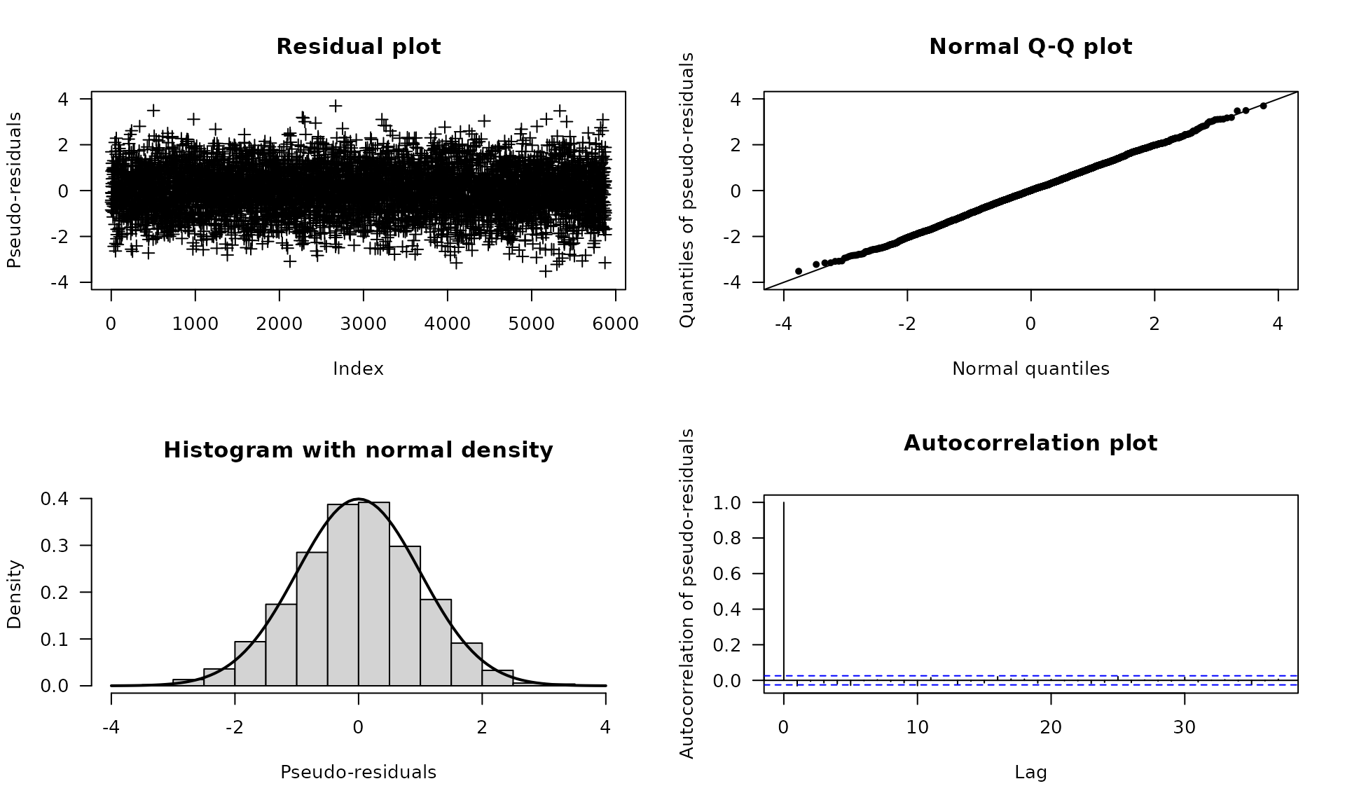

For additional normality tests, the residuals can be extracted from the model object via the residuals() method. The following lines exemplary perform a Jarque–Bera test (Jarque and Bera 1987):

tseries::jarque.bera.test(residuals(dax_model_3t))
#> 
#>  Jarque Bera Test
#> 
#> data:  residuals(dax_model_3t)
#> X-squared = 2.2403, df = 2, p-value = 0.3262

References

Jarque, C. M., and A. K. Bera. 1987. “A Test for Normality of Observations and Regression Residuals.” International Statistical Review / Revue Internationale de Statistique 55: 163–72.

Zucchini, W., I. L. MacDonald, and R. Langrock. 2016. “Hidden Markov Models for Time Series: An Introduction Using R, 2nd Edition.” Chapman and Hall/CRC.