State decoding and prediction

This vignette¹ introduces the Viterbi algorithm for state decoding. The decoded state sequence in combination with the estimated model parameters can be used for forecasting.

State decoding using the Viterbi algorithm

For financial markets, it is of special interest to infer the underlying (hidden) states in order to gain insight about the actual market situation. Decoding a full time series $S_1, \ldots, S_T$ is called global decoding. Hereby, we aim to find the most likely trajectory of hidden states under the estimated model. Global decoding can be accomplished by using the so-called Viterbi algorithm which is a recursive scheme enabling to find the global maximum without being confronted with huge computational costs. To this end, we follow Zucchini, MacDonald, and Langrock (2016) and define $$\zeta_{1i} = Pr(S_1 = i, X_1 = x_1) = \delta_i p_i(x_1)$$ for $i = 1, \ldots, N$ and for the following $t = 2, \ldots, T$$$\zeta_{ti} = \operatorname*{max}_{s_1, \ldots, s_{t-1}} Pr(S_{t-1} = s_{t-1}, S_t = i, X_t = x_t).$$ Then, the trajectory of most likely states $i_1, \ldots, i_T$ can be calculated recursively from $$i_T = \operatorname*{argmax}_{i = 1, \ldots, N} \zeta_{Ti}$$ and for the following $t = T-1, \ldots, 1$ from $$i_t = \operatorname*{argmax}_{i = 1, \ldots, N} (\zeta_{ti} \gamma_{i, i_{t+1}}).$$ Transferring the state decoding to HHMMs is straightforward: at first the coarse-scale state process must be decoded. Afterwards, by using this information the fine-scale state process can be decoded, see Adam et al. (2019).

The decode_states() function

We revisit the DAX model of the vignette on model estimation:

data(dax_model_3t)

The underlying states can be decoded via the decode_states() function:

dax_model_3t <- decode_states(dax_model_3t)
#> Decoded states

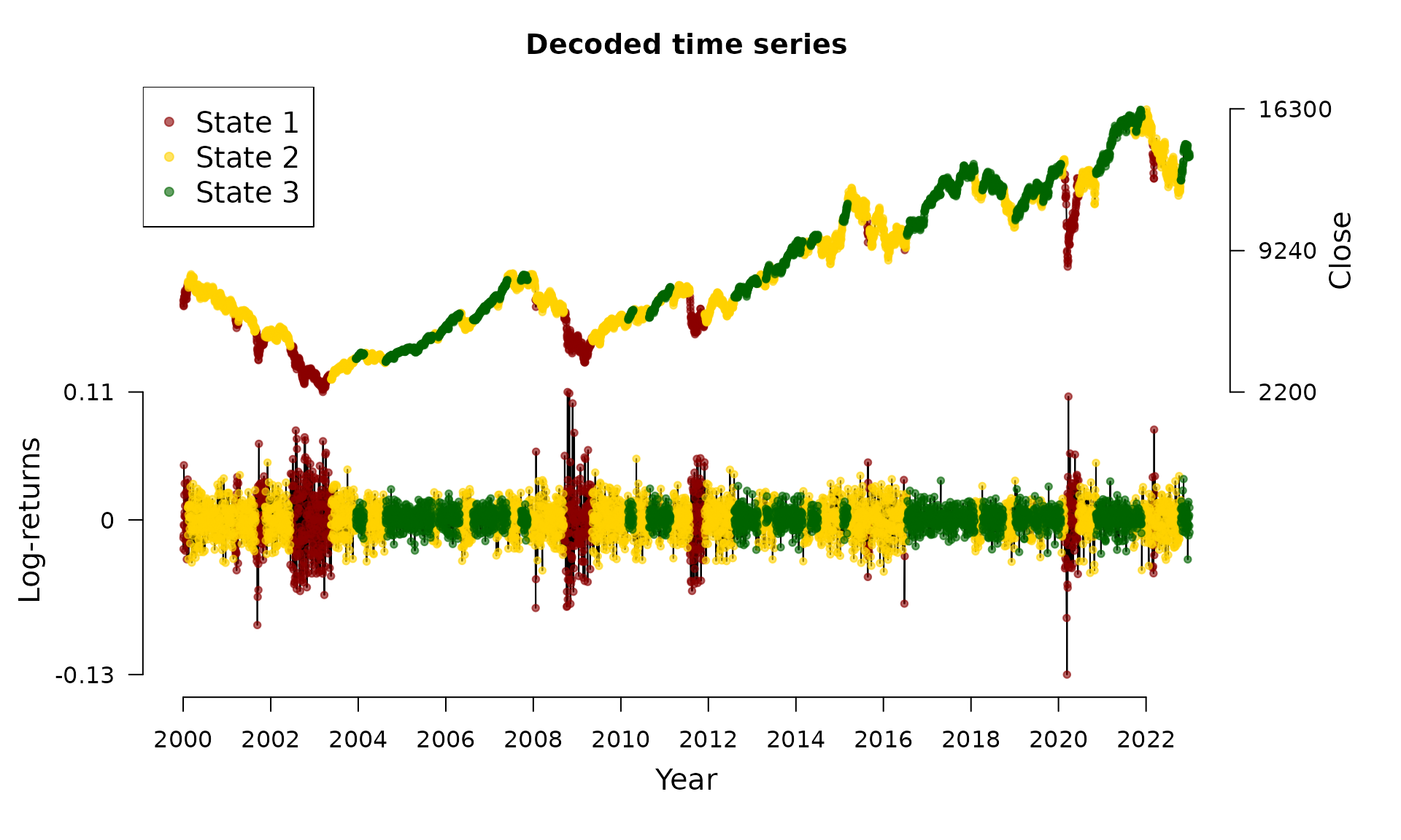
We now can visualize the decoded time series:

plot(dax_model_3t)

Invariance towards state labelling

Mind that the model is invariant to permutations of the state labels. Therefore, fHMM provides the option to switch labels after decoding via the reorder_states() function, for example:

dax_model_3t <- reorder_states(dax_model_3t, 3:1)

Prediction

Having decoded the underlying states, it is possible to compute the state probabilities of next observations. Based on these probabilities and in combination with the estimated state-dependent distributions, next observations can be predicted, compare Zucchini, MacDonald, and Langrock (2016):

predict(dax_model_3t, ahead = 10)
#>    state_1 state_2 state_3       lb estimate      ub
#> 1  0.00000 0.02446 0.97554 -0.01065  0.00123 0.01311
#> 2  0.00012 0.04773 0.95215 -0.01092  0.00120 0.01332
#> 3  0.00036 0.06988 0.92976 -0.01119  0.00116 0.01352
#> 4  0.00070 0.09095 0.90835 -0.01145  0.00113 0.01371
#> 5  0.00115 0.11099 0.88786 -0.01170  0.00110 0.01390
#> 6  0.00169 0.13006 0.86825 -0.01195  0.00107 0.01408
#> 7  0.00231 0.14821 0.84948 -0.01218  0.00104 0.01426
#> 8  0.00301 0.16547 0.83152 -0.01241  0.00101 0.01443
#> 9  0.00379 0.18189 0.81432 -0.01263  0.00098 0.01459
#> 10 0.00463 0.19751 0.79786 -0.01285  0.00095 0.01476

References

Adam, T., C. A. Griffiths, V. Leos-Barajas, E. N. Meese, C. G. Lowe, P. G. Blackwell, D. Righton, and R. Langrock. 2019. “Joint Modelling of Multi-Scale Animal Movement Data Using Hierarchical Hidden Markov Models.” Methods in Ecology and Evolution 10 (9): 1536–50.

Zucchini, W., I. L. MacDonald, and R. Langrock. 2016. “Hidden Markov Models for Time Series: An Introduction Using R, 2nd Edition.” Chapman and Hall/CRC.