Get started with RprobitB

Discrete choice models describe how a decider selects one alternative from a finite set, for example a train connection, an electricity supplier, or a mode of transport (Train 2009). The probability of each alternative is a function of the attributes of the alternatives and the characteristics of the decider. The coefficients of the model quantify the weight of each attribute in the decision, and ratios of coefficients quantify the trade-offs between attributes. RprobitB estimates discrete choice models in a Bayesian probit framework. This vignette fits a basic probit model to panel data from a stated choice experiment and introduces the posterior summaries, convergence diagnostics, and plots on which every analysis with the package relies.

The probit model

Consider $N$ deciders $n = 1, \dots, N$ , each of whom chooses at $T_n$ occasions $t = 1, \dots, T_n$ one of $J$ alternatives $j = 1, \dots, J$ . The probit model is a random utility model: it assigns to every alternative the latent utility

$U_{ntj} = X_{ntj}^\top \beta_n + \epsilon_{ntj}, \qquad \epsilon_{nt} = (\epsilon_{nt1}, \dots, \epsilon_{ntJ})^\top \sim \mathrm{N}(0, \Sigma),$

where $X_{ntj}$ is the vector of $P$ covariates assigned to alternative $j$ at occasion $t$ of decider $n$ , $\beta_n$ is the vector of the $P$ coefficients of decider $n$ , and $\epsilon_{ntj}$ is an error term. The error vector $\epsilon_{nt}$ of an occasion is multivariate normal with mean zero and the $J \times J$ covariance matrix $\Sigma$ , and it is independent across deciders and occasions. The decider chooses the alternative with the largest utility, $y_{nt} = \operatorname{argmax}_j U_{ntj}$ , and only this choice $y_{nt}$ is observed, not the utilities. The choice probability of alternative $j$ is the probability that its utility exceeds the utilities of all other alternatives,

$\Pr(y_{nt} = j) = \Pr(U_{ntj} > U_{ntl} \text{ for all } l \neq j),$

which is a function of the covariates $X_{nt}$ of the occasion, the coefficients $\beta_n$ , and the covariance matrix $\Sigma$ . The choice probabilities are invariant to adding a constant to all utilities and to multiplying all utilities by a positive number, so neither the level nor the scale of the utilities is identified. RprobitB removes the level by taking utility differences with respect to a base alternative and fixes the scale by restricting either one error variance or one coefficient. These two restrictions are the normalization of the model. The coefficient vector $\beta_n$ is common to all deciders unless random effects are specified, in which case the coefficients of every decider are drawn from a population distribution whose parameters are estimated. The vignette Model specification and variants describes the normalization and the prior distribution, and the vignette Modeling preference heterogeneity the specification of heterogeneous coefficients. Bayesian estimation of the multinomial probit model goes back to McCulloch and Rossi (1994) and Imai and van Dyk (2005), and Oelschläger (2026) gives a unified account of the heterogeneity models that RprobitB implements.

A stated choice experiment on train trips

In 1987, a stated choice experiment commissioned by the Dutch national railways presented 235 travelers with pairs of hypothetical train trips and asked which trip of each pair they would choose (Ben-Akiva et al. 1993). The two trips of a pair differ in price, travel time, number of changes, and comfort class, and every traveler evaluated about twelve pairs. The mlogit package (Croissant 2020) provides the 2929 choices as the data set Train. The data are in wide format: one row per choice occasion, with the attributes of trip A in the columns ending in _A and those of trip B in the columns ending in _B. Prices are recorded in cents of Dutch guilders and travel times in minutes; both are converted to euro and hours below.

library(RprobitB)
set.seed(1)
data("Train", package = "mlogit")
Train$price_A <- Train$price_A / 100 / 2.20371
Train$price_B <- Train$price_B / 100 / 2.20371
Train$time_A <- Train$time_A / 60
Train$time_B <- Train$time_B / 60
head(Train)
#>   choiceid id choice  price_A  price_B   time_A   time_B change_A change_B
#> 1        1  1      A 10.89073 18.15121 2.500000 2.500000        0        0
#> 2        2  1      A 10.89073 14.52097 2.500000 2.166667        0        0
#> 3        3  1      A 10.89073 18.15121 1.916667 1.916667        0        0
#> 4        4  1      B 18.15121 14.52097 2.166667 2.500000        0        0
#> 5        5  1      B 10.89073 14.52097 2.500000 2.500000        0        0
#> 6        6  1      B 18.15121 10.89073 1.916667 2.166667        0        0
#>   comfort_A comfort_B
#> 1         1         1
#> 2         1         1
#> 3         1         0
#> 4         1         0
#> 5         1         0
#> 6         0         0

The model formula names the response and the covariates:

formula <- choice ~ price + time + change + factor(comfort) | 0

All four covariates are attributes of the trips with one coefficient common to both alternatives, which places them in the first part of the formula. The second part takes characteristics of the decider and the alternative-specific constants; here it contains only the 0 that removes the constants, which is appropriate because the labels A and B of the two trips were assigned arbitrarily and carry no utility of their own. The comfort class is stored as an integer but is a categorical variable with three levels; factor(comfort) expands it into dummy variables, as in lm(). The arguments column_decider and column_occasion identify the traveler and the choice occasion. The vignette Model specification and variants describes the three parts of the formula and the further arguments of fit().

model <- fit(
  formula = formula,
  data = Train,
  column_decider = "id",
  column_occasion = "choiceid",
  iterations = 2000,
  warmup = 1000,
  chains = 2,
  progress = FALSE
)
model
#> Bayesian probit choice model
#> Formula: choice ~ price + time + change + factor(comfort) | 0 | 0 
#> Data: 235 deciders, 2929 choice occasions
#> Samples: 1000 retained per chain, 2 chains

fit() estimates the model with a Gibbs sampler, a Markov chain Monte Carlo method that draws the latent utilities and the parameters in turn from their conditional posterior distributions. The posterior distribution combines the prior distribution of the parameters, described in the vignette Model specification and variants, with the likelihood of the observed choices. A chain of the sampler consists of iterations draws. The first warmup of them are discarded, because the chain first has to move from its starting values into the region of the posterior, and the remaining draws are retained as the posterior draws from which every summary below is computed. Several independent chains, set by chains, sample the same posterior and make it possible to check convergence, that is, whether the retained draws represent the posterior distribution.

Posterior summaries

summary() reports the posterior mean, mode, and standard deviation of every population-level parameter together with the convergence diagnostics of the posterior package (Bürkner et al. 2026).

summary(model)
#> Bayesian probit choice model
#> Formula: choice ~ price + time + change + factor(comfort) | 0 | 0 
#> Samples: 1000 retained per chain, 2 chains
#> 
#>                variable   mean   mode      sd rhat ess_bulk
#>             beta[price] -0.196 -0.196 0.00873 1.01      349
#>              beta[time] -1.054 -1.047 0.09503 1.00      596
#>            beta[change] -0.201 -0.208 0.03580 1.01      657
#>  beta[factor(comfort)1] -0.396 -0.396 0.04300 1.00      800
#>  beta[factor(comfort)2] -1.338 -1.320 0.07954 1.01      553

The coefficients of price, travel time, and number of changes are negative, as expected: each of these attributes reduces the utility of a trip. Comfort is a factor whose level 0 denotes the highest class, so the negative coefficients of the dummies for levels 1 and 2 quantify the loss of utility in the lower classes. The error variance of the utility difference, Sigma[B,B], is absent from the table because the default normalization fixes it to one.

Because of this normalization, the coefficients are measured in units of the error standard deviation, and their absolute size has no substantive interpretation. The ratio of two coefficients is invariant to the scale and answers a substantive question: which price reduction compensates a traveler for one additional hour of travel time? interpret() computes such ratios for every posterior draw and expresses each effect in units of a reference effect, here the price:

compensation <- interpret(model, reference = "price")
compensation
#> 1 `time` compensates -5.38 `price` (95% interval -6.18 to -4.51)
#> 1 `change` compensates -1.03 `price` (95% interval -1.37 to -0.677)
#> 1 `factor(comfort)1` compensates -2.02 `price` (95% interval -2.42 to -1.62)
#> 1 `factor(comfort)2` compensates -6.83 `price` (95% interval -7.6 to -6.09)

One additional hour of travel time is compensated by a price that is about 5.4 euro lower (at 1987 prices), and the lowest comfort class relative to the highest by a price about 6.8 euro lower.

The last two columns of the summary table are the convergence diagnostics recommended by Vehtari et al. (2021):

rhat compares the variance between the chains with the variance within the chains and equals one when all chains sample the same distribution.
ess_bulk is the effective sample size for the bulk of the posterior distribution, that is, for its central part around the median as opposed to its tails. Consecutive draws of a chain are correlated, and the effective sample size is the number of independent draws that would estimate the posterior mean or median with the same precision. A few hundred effective draws suffice for these summaries; the precision of extreme quantiles is governed by the tail effective sample size instead.

The arguments probs and statistics select the columns of the table. probs adds posterior quantiles, and statistics selects the measures, among them the tail effective sample size, which governs the precision of the quantiles, and the Monte Carlo standard error of the mean, which quantifies the simulation error of the reported posterior mean. ?summary.RprobitB_fit describes each measure.

summary(
  model,
  statistics = c("mean", "mcse_mean", "ess_bulk", "ess_tail"),
  probs = c(0.05, 0.95)
)
#> Bayesian probit choice model
#> Formula: choice ~ price + time + change + factor(comfort) | 0 | 0 
#> Samples: 1000 retained per chain, 2 chains
#> 
#>                variable   mean     q5    q95 mcse_mean ess_bulk ess_tail
#>             beta[price] -0.196 -0.210 -0.182  0.000468      349      811
#>              beta[time] -1.054 -1.209 -0.897  0.003890      596      923
#>            beta[change] -0.201 -0.260 -0.141  0.001397      657     1251
#>  beta[factor(comfort)1] -0.396 -0.469 -0.323  0.001520      800     1186
#>  beta[factor(comfort)2] -1.338 -1.469 -1.207  0.003376      553     1056

coef() and confint() return posterior means or medians and equal-tailed credible intervals. The bounds of such an interval are the posterior quantiles at (1 - level) / 2 and (1 + level) / 2, so that the interval contains the parameter with posterior probability level.

coef(model)
#>            beta[price]             beta[time]           beta[change] 
#>             -0.1961137             -1.0541476             -0.2013516 
#> beta[factor(comfort)1] beta[factor(comfort)2] 
#>             -0.3961042             -1.3382782
confint(model, level = 0.9)
#>                                5%        95%
#> beta[price]            -0.2101777 -0.1819134
#> beta[time]             -1.2093530 -0.8967781
#> beta[change]           -0.2596503 -0.1410680
#> beta[factor(comfort)1] -0.4688508 -0.3233941
#> beta[factor(comfort)2] -1.4687676 -1.2068223

vcov() returns the posterior covariance matrix of the parameters:

round(vcov(model), 5)
#>                        beta[price] beta[time] beta[change]
#> beta[price]                0.00008    0.00037      0.00008
#> beta[time]                 0.00037    0.00903      0.00083
#> beta[change]               0.00008    0.00083      0.00128
#> beta[factor(comfort)1]     0.00014    0.00123      0.00024
#> beta[factor(comfort)2]     0.00031    0.00301      0.00061
#>                        beta[factor(comfort)1] beta[factor(comfort)2]
#> beta[price]                           0.00014                0.00031
#> beta[time]                            0.00123                0.00301
#> beta[change]                          0.00024                0.00061
#> beta[factor(comfort)1]                0.00185                0.00216
#> beta[factor(comfort)2]                0.00216                0.00633

An interval plot displays the marginal posteriors: the thick bars cover the central 50% and the thin lines the central 90% of each posterior.

plot(model, type = "interval")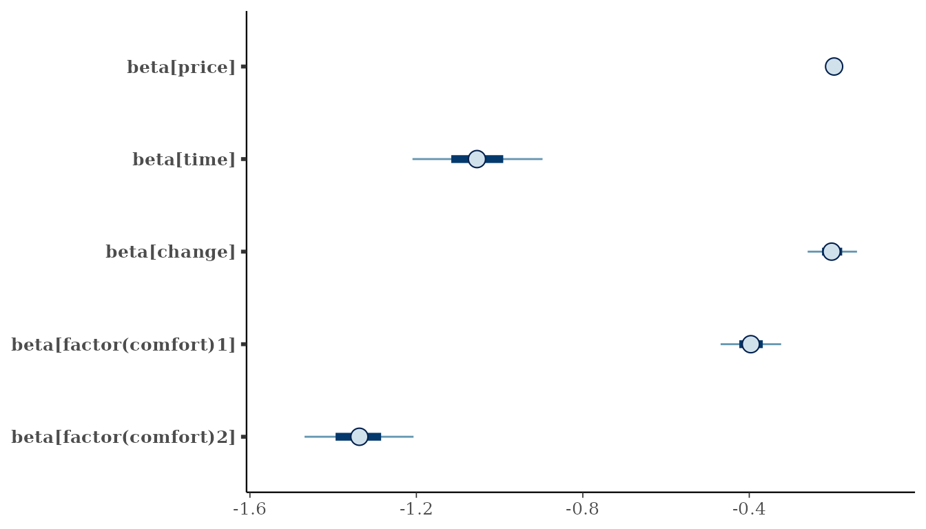

Graphical convergence diagnostics

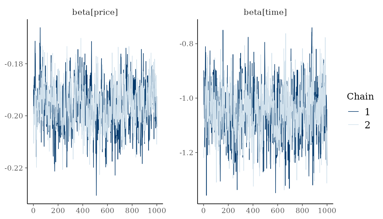
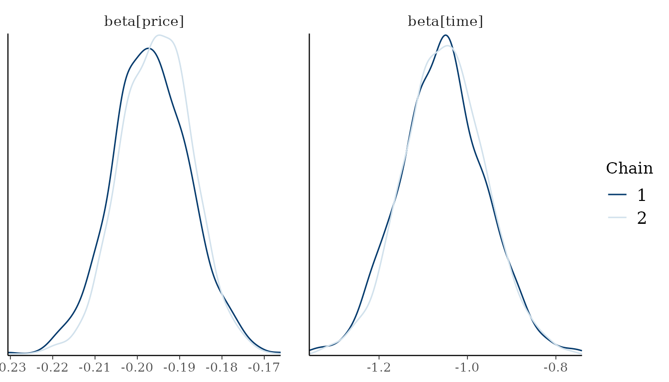
plot() delegates to bayesplot (Gabry and Mahr 2025). Trace plots show the draws of each chain against their index, and density overlays compare the marginal posteriors of the chains; there are two chains here because fit() was called with chains = 2. For converged chains, the traces are stationary without trend, and the densities of the chains coincide.

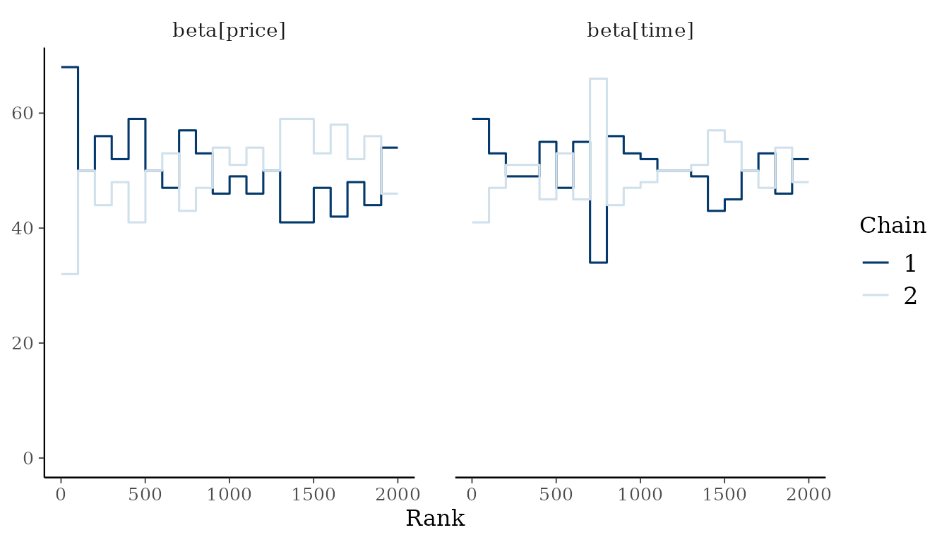
plot(model, type = "trace", variables = c("beta[price]", "beta[time]"))

plot(model, type = "density", variables = c("beta[price]", "beta[time]"))

Rank plots are a more sensitive check (Vehtari et al. 2021). The draws of all chains are pooled and ranked, and the histogram of the ranks is drawn for every chain. If all chains sample the same distribution, every chain receives ranks from the whole range with equal frequency, and the histograms are uniform. A chain that remains in a subregion of the posterior, for example because it has not yet left the region of its starting values, receives predominantly small or large ranks, and its histogram is peaked at one end.

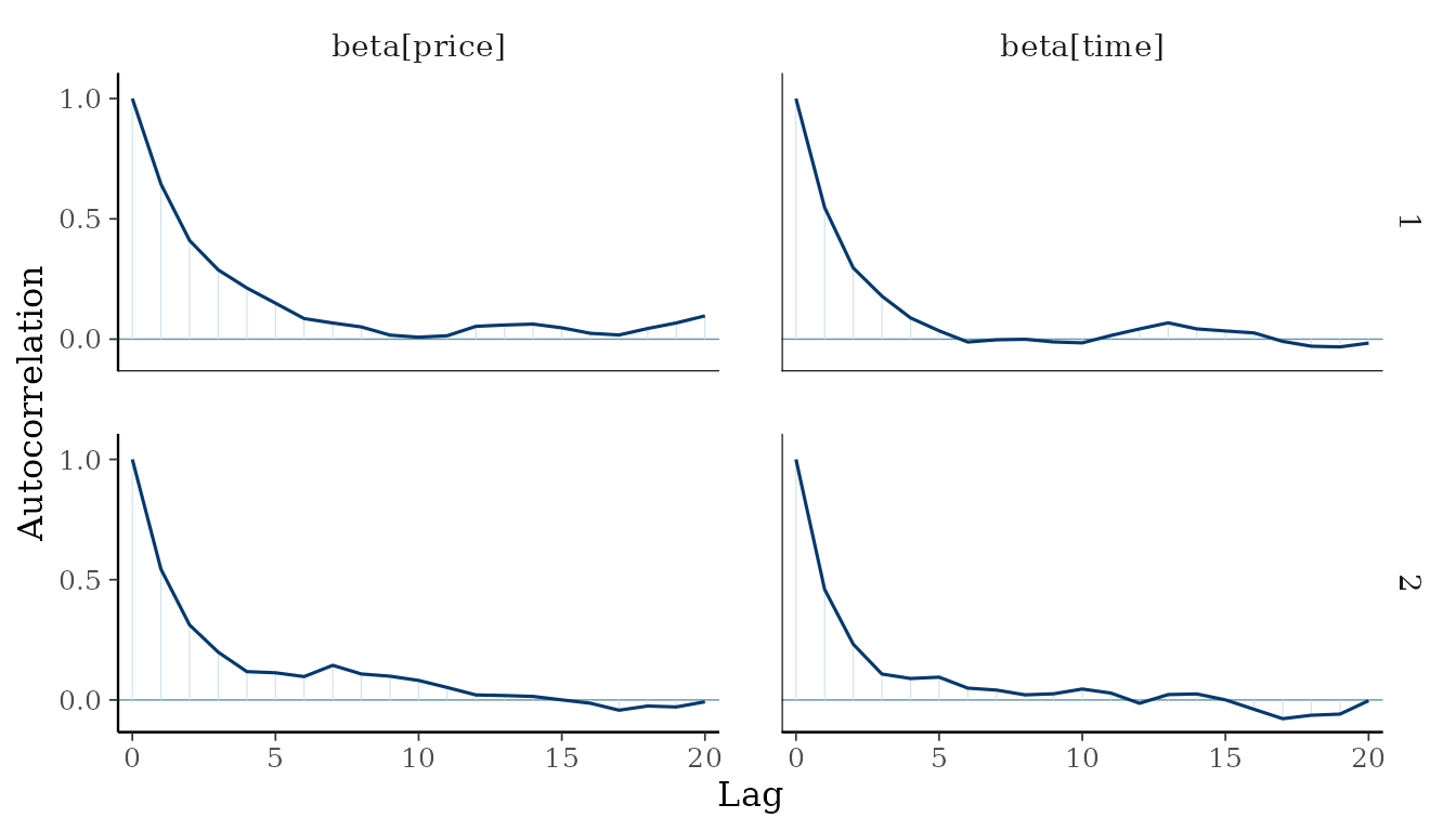
Autocorrelation plots show, for every chain, the correlation between draws that are $k$ iterations apart as a function of the lag $k$ . Consecutive draws of a Gibbs sampler are dependent, so a chain carries less information than the same number of independent draws. The effective sample size expresses this loss in one number: it is the number of independent draws that would estimate the posterior mean with the same precision. In its classical form, it equals $S / (1 + 2 \sum_{k \geq 1} \rho_k)$ for $S$ draws with autocorrelations $\rho_k$ , so the faster the autocorrelation decays to zero, the closer the effective sample size is to the number of draws. ess_bulk applies this formula to rank-normalized draws, which makes it robust to heavy tails (Vehtari et al. 2021).

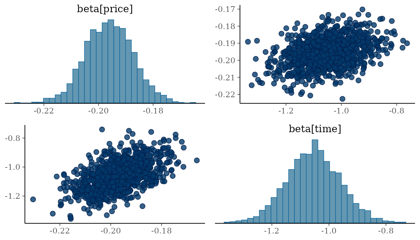
plot(model, type = "rank", variables = c("beta[price]", "beta[time]"))

plot(model, type = "acf", variables = c("beta[price]", "beta[time]"))

Pairs plots show the joint posterior of two parameters and reveal posterior correlations:

plot(model, type = "pairs", variables = c("beta[price]", "beta[time]"))

Working with the posterior draws

The retained draws are stored as a draws_array of the posterior package with dimensions iteration, chain, and variable, so that all functions of that package apply to them directly.

draws <- posterior::as_draws(model)
dim(draws)
#> [1] 1000    2    6
posterior::summarise_draws(draws, "mean", "quantile2")
#> # A tibble: 6 × 4
#>   variable                 mean     q5    q95
#>   <chr>                   <dbl>  <dbl>  <dbl>
#> 1 beta[price]            -0.196 -0.210 -0.182
#> 2 beta[time]             -1.05  -1.21  -0.897
#> 3 beta[change]           -0.201 -0.260 -0.141
#> 4 beta[factor(comfort)1] -0.396 -0.469 -0.323
#> 5 beta[factor(comfort)2] -1.34  -1.47  -1.21 
#> 6 Sigma[B,B]              1      1      1

The standard accessor methods are available: formula() returns the fitted formula, model.frame() the data the model was fitted to, and nobs() the number of independent units in the likelihood. Here these are the observed choice occasions, because the model has one coefficient vector for all travelers. With random effects, and with the latent classes of the vignette Modeling preference heterogeneity, the choices of a traveler are dependent, and nobs() counts travelers.

formula(model)
#> choice ~ price + time + change + factor(comfort) | 0 | 0
nobs(model)
#> [1] 2929
head(model.frame(model))
#>   id choiceid choice  price_A  price_B   time_A   time_B change_A change_B
#> 1  1        1      A 10.89073 18.15121 2.500000 2.500000        0        0
#> 2  1        2      A 10.89073 14.52097 2.500000 2.166667        0        0
#> 3  1        3      A 10.89073 18.15121 1.916667 1.916667        0        0
#> 4  1        4      B 18.15121 14.52097 2.166667 2.500000        0        0
#> 5  1        5      B 10.89073 14.52097 2.500000 2.500000        0        0
#> 6  1        6      B 18.15121 10.89073 1.916667 2.166667        0        0
#>   comfort_A comfort_B
#> 1         1         1
#> 2         1         1
#> 3         1         0
#> 4         1         0
#> 5         1         0
#> 6         0         0

Parallel chains

The chains of a fit are independent of each other, so RprobitB can run them in parallel on several cores, which reduces the computing time in proportion to the number of chains. The package does not select a parallel backend itself. The chains run through the future framework (Bengtsson 2021), so a plan set before fitting is used automatically.

future::plan(future::multisession, workers = 4) # run chains on four cores
parallel_model <- fit(
  formula = formula,
  data = Train,
  column_decider = "id",
  column_occasion = "choiceid"
)
future::plan(future::sequential) # return to sequential evaluation

In interactive sessions, all chains report their progress through the progressr package (Bengtsson 2026).

References

Ben-Akiva, Moshe, Denis Bolduc, and Mark Bradley. 1993. “Estimation of Travel Choice Models with Randomly Distributed Values of Time.” Transportation Research Record 1413: 88–97. https://trid.trb.org/View/385096.

Bengtsson, Henrik. 2021. “A Unifying Framework for Parallel and Distributed Processing in R Using Futures.” The R Journal 13 (2): 208–27. https://doi.org/10.32614/RJ-2021-048.

Bengtsson, Henrik. 2026. progressr: An Inclusive, Unifying API for Progress Updates. https://doi.org/10.32614/CRAN.package.progressr.

Bürkner, Paul-Christian, Jonah Gabry, Matthew Kay, and Aki Vehtari. 2026. posterior: Tools for Working with Posterior Distributions. https://mc-stan.org/posterior/.

Croissant, Yves. 2020. “Estimation of Random Utility Models in R: The mlogit Package.” Journal of Statistical Software 95 (11): 1–41. https://doi.org/10.18637/jss.v095.i11.

Gabry, Jonah, and Tristan Mahr. 2025. bayesplot: Plotting for Bayesian Models. https://mc-stan.org/bayesplot/.

Imai, Kosuke, and David A. van Dyk. 2005. “A Bayesian Analysis of the Multinomial Probit Model Using Marginal Data Augmentation.” Journal of Econometrics 124 (2): 311–34. https://doi.org/10.1016/j.jeconom.2004.02.002.

McCulloch, Robert E., and Peter E. Rossi. 1994. “An Exact Likelihood Analysis of the Multinomial Probit Model.” Journal of Econometrics 64 (1-2): 207–40. https://doi.org/10.1016/0304-4076(94)90064-7.

Oelschläger, Lennart. 2026. “Overcoming Challenges in Modeling Choice Behavior Heterogeneity.” PhD thesis, Bielefeld University. https://pub.uni-bielefeld.de/record/3014719.

Train, Kenneth E. 2009. Discrete Choice Methods with Simulation. 2nd ed. Cambridge University Press. https://doi.org/10.1017/CBO9780511805271.

Vehtari, Aki, Andrew Gelman, Daniel Simpson, Bob Carpenter, and Paul-Christian Bürkner. 2021. “Rank-Normalization, Folding, and Localization: An Improved

\widehat{R}

for Assessing Convergence of MCMC.” Bayesian Analysis 16 (2): 667–718. https://doi.org/10.1214/20-BA1221.