
A fitted choice model answers questions about choice probabilities:
which of two train trips a traveler is likely to book, how the support
for a wind-power project changes with the compensation, and how well the
model predicts the choices of deciders that were not used for
estimation. In the probit model introduced in the vignette Get
started with RprobitB, the choice probability of an alternative is
the probability that its latent utility exceeds the utilities of the
other alternatives, and it depends on the covariates of the occasion and
on the parameters. predict() evaluates these probabilities
under every retained posterior draw and averages them, so that the
predictions account for the posterior uncertainty about the parameters
(Gelman et al.
1996). This vignette covers predictions for the population
and for individual deciders, scenarios, out-of-sample prediction,
residuals, and marginal effects. The examples use data sets of the
mlogit package (Croissant 2020), the
choicedata package (Oelschläger 2026), and the
MASS package (Venables and Ripley 2002).
A random price coefficient
The Train data of the mlogit package
contain about a dozen choices by each of 235 Dutch travelers between two
hypothetical train trips that differ in price, travel time, number of
changes, and comfort class (Ben-Akiva et al. 1993). As in the
vignette Get
started with RprobitB, the prices are converted to euro and the
travel times to hours. That vignette fits one price coefficient for all
travelers. Here the price coefficient is a normal random effect, as
introduced in the vignette Modeling
preference heterogeneity: every traveler has an individual price
coefficient, drawn from a normal population distribution whose mean and
variance are estimated. The fit uses the first 100 travelers. The
individual draws are saved because the conditional predictions below use
them, and thinning keeps 100 draws in total, which keeps the predictions
fast.
data("Train", package = "mlogit")
Train$price_A <- Train$price_A / 100 / 2.20371
Train$price_B <- Train$price_B / 100 / 2.20371
Train$time_A <- Train$time_A / 60
Train$time_B <- Train$time_B / 60
train_small <- Train[Train$id %in% unique(Train$id)[1:100], ]
model <- fit(
  choice ~ price + time + change + factor(comfort) | 0,
  data = train_small,
  random_effects = "price",
  column_decider = "id",
  column_occasion = "choiceid",
  iterations = 1500,
  warmup = 750,
  thin = 15,
  chains = 2,
  save_individual_draws = TRUE,
  progress = FALSE
)
summary(model)
#> Bayesian probit choice model
#> Formula: choice ~ price + time + change + factor(comfort) | 0 | 0
#> Samples: 50 retained per chain, 2 chains
#>
#>                variable   mean   mode     sd  rhat ess_bulk
#>              beta[time] -2.052 -1.994 0.1633 0.997    102.5
#>            beta[change] -0.358 -0.331 0.0644 1.038     99.3
#>  beta[factor(comfort)1] -0.659 -0.646 0.0823 1.016     82.5
#>  beta[factor(comfort)2] -2.124 -2.165 0.1619 1.023     81.4
#>               mu[price] -0.453 -0.449 0.0490 1.024    102.1
#>      Omega[price,price]  0.136  0.123 0.0279 1.054     39.2
mu[price] and Omega[price,price] are the
mean and the variance of the price coefficient across the population.
Price sensitivity differs considerably between travelers, which the
predictions below take into account.
Population predictions
By default, predict() returns one row per choice
occasion with the identifiers, the most probable alternative in
.prediction, and the posterior mean probability of every
alternative. These population predictions integrate over the estimated
population distribution of the random coefficient, so they apply to any
traveler from the population.
population <- predict(model)
head(population)
#>   id choiceid .prediction probability_A probability_B
#> 1  1        1           A     0.8751930     0.1248070
#> 2  1        2           A     0.7171419     0.2828581
#> 3  1        3           A     0.8216767     0.1783233
#> 4  1        4           B     0.1667812     0.8332188
#> 5  1        5           A     0.7221889     0.2778111
#> 6  1        6           B     0.1653464     0.8346536
uncertainty = TRUE adds the posterior standard deviation
and an equal-tailed credible interval of every probability, here at the
90% level. The intervals reflect the posterior uncertainty about the
parameters.
head(predict(model, uncertainty = TRUE, level = 0.9))
#>   id choiceid .prediction probability_A probability_B       sd_A       sd_B
#> 1  1        1           A     0.8751930     0.1248070 0.02950544 0.02950544
#> 2  1        2           A     0.7171419     0.2828581 0.03370647 0.03370647
#> 3  1        3           A     0.8216767     0.1783233 0.03421977 0.03421977
#> 4  1        4           B     0.1667812     0.8332188 0.02966028 0.02966028
#> 5  1        5           A     0.7221889     0.2778111 0.03525608 0.03525608
#> 6  1        6           B     0.1653464     0.8346536 0.03293069 0.03293069
#>     lower_A    lower_B   upper_A   upper_B
#> 1 0.8200832 0.08765568 0.9123443 0.1799168
#> 2 0.6601476 0.24004918 0.7599508 0.3398524
#> 3 0.7591170 0.13404372 0.8659563 0.2408830
#> 4 0.1295135 0.77544068 0.2245593 0.8704865
#> 5 0.6591562 0.23266991 0.7673301 0.3408438
#> 6 0.1223764 0.77477653 0.2252235 0.8776236
Conditional predictions for fitted deciders
The dozen choices of a traveler are informative about their
individual price coefficient. coef(level = "individual")
returns the posterior mean of every traveler’s coefficient, and
predict(type = "conditional") uses the individual draws
instead of the population distribution. Conditional predictions exist
only for the deciders in the fitted data, and they are usually sharper
because they use the decider’s own choices. This partial pooling is the
main argument for hierarchical Bayesian choice models (Allenby and Rossi 1998;
Huber and Train 2001).
head(coef(model, level = "individual"))
#>         price
#> 1 -0.27257169
#> 2 -0.81931599
#> 3 -0.72985640
#> 4 -0.49340645
#> 5 -0.01806365
#> 6 -0.06974627
conditional <- predict(model, type = "conditional")
head(conditional)
#>   id choiceid .prediction probability_A probability_B
#> 1  1        1           A     0.9547870     0.0452130
#> 2  1        2           A     0.6144646     0.3855354
#> 3  1        3           A     0.8702504     0.1297496
#> 4  1        4           B     0.1800033     0.8199967
#> 5  1        5           A     0.6239918     0.3760082
#> 6  1        6           B     0.1060654     0.8939346
The hit rate, the share of correctly predicted choices in the fitted data, is one measure of the gain:
observed <- model.frame(model)$choice
c(
  population = mean(population$.prediction == observed, na.rm = TRUE),
  conditional = mean(conditional$.prediction == observed, na.rm = TRUE)
)
#>  population conditional
#>   0.7370968   0.8153226
The hit rate evaluates the predictions at a single threshold, a
probability of one half. An ROC curve compares them at every threshold:
as the threshold for predicting trip B decreases from one
to zero, the curve plots the share of B choices predicted
correctly against the share of A choices wrongly predicted
as B. The plotROC package (Sachs 2017) draws
the curves with ggplot2 (Wickham 2016).
library(ggplot2)
library(plotROC)
roc_data <- rbind(
  data.frame(
    prediction = "population", chose_B = as.integer(observed == "B"),
    probability = population$probability_B
  ),
  data.frame(
    prediction = "conditional", chose_B = as.integer(observed == "B"),
    probability = conditional$probability_B
  )
)
roc_data$prediction <- factor(
  roc_data$prediction, levels = c("population", "conditional")
)
roc_plot <- ggplot(
  roc_data, aes(d = chose_B, m = probability, color = prediction)
) +
  geom_roc(n.cuts = 0) +
  style_roc()
roc_plot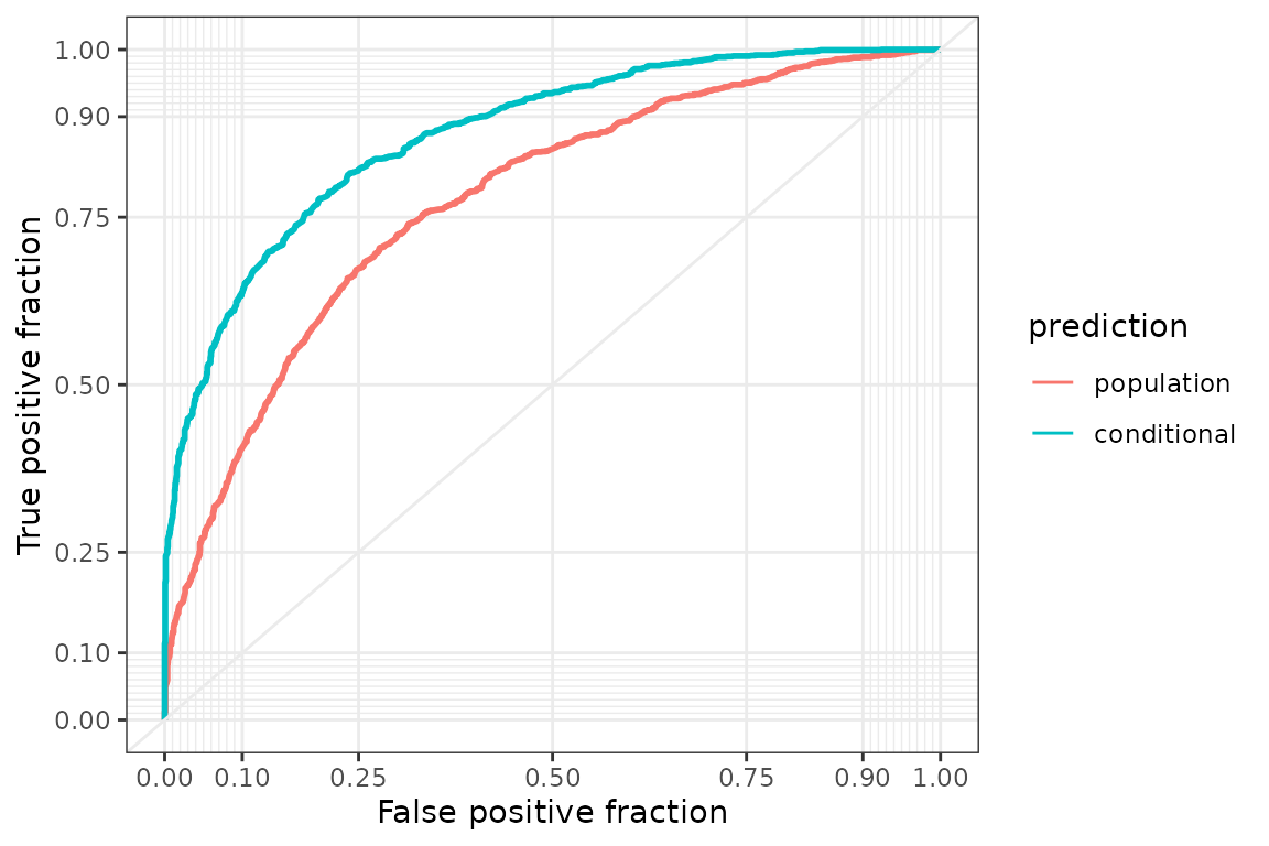
The conditional curve lies above the population curve and therefore has the larger area under the curve, which equals one for a perfect and one half for an uninformative prediction.
Scenario analysis in a stated choice experiment
A scenario predicts the choice probabilities for modified attributes.
Near Setskog in Norway, 308 residents were asked six times to choose
between two plans for a proposed wind-power project and the status quo
without the project, alternative 1 (Dugstad et al.
2024). The plans varied the number and height of the
turbines, the routing of the power line, and an annual reduction in
municipal taxes offered as compensation. The study also measured each
respondent’s collective psychological ownership of the affected area, a
standardized score of how strongly they feel that the landscape belongs
to the residents. The score does not vary across alternatives and
therefore enters the second part of the formula, which gives it one
coefficient per plan relative to the status quo. The fit uses the first
150 respondents.
wind_formula <- choice ~ turbines + height + powerline + compensation |
  psychological_ownership
data("wind_power_choice", package = "choicedata")
respondents <- unique(wind_power_choice$respondent)[1:150]
wind_small <- wind_power_choice[
  wind_power_choice$respondent %in% respondents,
]
wind <- fit(
  formula = wind_formula,
  data = wind_small,
  column_decider = "respondent",
  column_occasion = "occasion",
  iterations = 10000,
  warmup = 5000,
  thin = 10,
  chains = 1,
  progress = FALSE
)
coef(wind)[c("beta[compensation]", "beta[psychological_ownership_2]")]
#>              beta[compensation] beta[psychological_ownership_2]
#>                     0.001224175                    -0.486325523
The compensation coefficient is positive and the ownership coefficient negative: compensation makes a plan more attractive, and residents with a stronger feeling of ownership are less willing to leave the status quo.
What would happen if the municipality doubled the compensation?
newdata accepts a data frame in the layout of the fitted
data, with or without the response column. The scenario below doubles
the compensation of both plans in the first four choice tasks and
compares the probability of the status quo before and after.
tasks <- model.frame(wind)[1:4, ]
tasks$choice <- NULL
scenario <- tasks
scenario$compensation_2 <- 2 * scenario$compensation_2
scenario$compensation_3 <- 2 * scenario$compensation_3
cbind(
  before = predict(wind, newdata = tasks)$probability_1,
  after = predict(wind, newdata = scenario)$probability_1
)
#>         before     after
#> [1,] 0.3164275 0.1813277
#> [2,] 0.2890407 0.1832128
#> [3,] 0.2924634 0.2202136
#> [4,] 0.3524318 0.2807522
Doubling the compensation lowers the probability of the status quo in all four tasks.
Out-of-sample prediction and calibration
Predictive performance is best judged on deciders that were not used
for estimation (Vehtari et al. 2017). In an arena
tournament on the chess server Lichess, a player may go Berserk at the
start of a game: the clock is halved, and a win earns one extra
tournament point. Players on a winning streak collect double points, so
a loss is more costly for them. The lichess_berserk_choice
data of the choicedata package record this decision for
5852 players in the Lichess Yearly Rapid Arena of April 2026, game by
game, together with the playing color, the player’s rating, the rating
difference to the opponent, the remaining tournament time, and whether
the player was on a streak. All covariates describe the game and are
constant across the two alternatives, so they enter the second part of
the formula, which gives each of them one coefficient for the
alternative TRUE relative to FALSE, for
example beta[rating_TRUE]. Logical covariates appear as
dummy variables such as streakTRUE.
berserk_formula <- berserk ~ 0 | white + rating + ratingDifference +
  minutesRemaining + streak
The fit uses the games of the first 300 players.
train_test() splits them by decider:
test_number = 60 puts all games of 60 players into the test
set and the games of the other players into the training set.
data("lichess_berserk_choice", package = "choicedata")
players <- unique(lichess_berserk_choice$deciderID)
first_players <- lichess_berserk_choice$deciderID %in% players[1:300]
split <- train_test(lichess_berserk_choice[first_players, ], test_number = 60)
berserk <- fit(
  formula = berserk_formula,
  data = split$train,
  column_occasion = "occasionID",
  iterations = 1000,
  warmup = 500,
  chains = 2,
  progress = FALSE
)
coef(berserk)
#>        beta[whiteTRUE_TRUE]           beta[rating_TRUE]
#>                0.0326143683                0.0014833175
#> beta[ratingDifference_TRUE] beta[minutesRemaining_TRUE]
#>                0.0000604789               -0.0001783328
#>       beta[streakTRUE_TRUE]              beta[ASC_TRUE]
#>               -0.0734418466               -3.2266432134
The rating coefficient is positive: stronger players go Berserk more
often. The coefficients of the streak and of the remaining time are
negative. How well does the model predict the games of the 60 players in
the test set? newdata takes the test set as it is, and the
predicted alternative is compared with the observed one.
holdout_prediction <- predict(berserk, newdata = split$test)
holdout_choice <- as.character(split$test$berserk)
c(
  accuracy = mean(holdout_prediction$.prediction == holdout_choice),
  share_berserk = mean(split$test$berserk)
)
#>      accuracy share_berserk
#>     0.6810700     0.3497942
The hit rate is only slightly higher than the share of games without Berserk, which the rule that never predicts Berserk would already reach, so the hit rate alone is a weak criterion for an unbalanced binary response. A calibration analysis assesses the predicted probabilities instead. It groups the hold-out games by predicted Berserk probability in intervals of width 0.1 and compares the mean predicted probability with the observed Berserk rate in each group; groups with fewer than 50 games are dropped.
predicted <- holdout_prediction$probability_TRUE
bins <- cut(predicted, breaks = seq(0, 1, by = 0.1))
calibration <- data.frame(
  games = as.vector(table(bins)),
  predicted = as.vector(tapply(predicted, bins, mean)),
  observed = as.vector(tapply(split$test$berserk, bins, mean)),
  row.names = levels(bins)
)
large <- calibration[calibration$games >= 50, ]
round(large, 2)
#>           games predicted observed
#> (0.1,0.2]    57      0.14     0.18
#> (0.2,0.3]   202      0.25     0.25
#> (0.3,0.4]    74      0.35     0.35
#> (0.4,0.5]    81      0.43     0.57
The calibration plot shows the same table. Points on the diagonal mean that the predicted probability equals the observed rate, and the point sizes are proportional to the number of games in a group.
plot(
  large$predicted, large$observed,
  xlim = c(0, 1), ylim = c(0, 1), pch = 19,
  cex = 0.5 + 2 * large$games / max(large$games),
  xlab = "predicted Berserk probability",
  ylab = "observed Berserk rate"
)
abline(0, 1, lwd = 2, col = "grey50")
The observed Berserk rate rises with the predicted probability, so the model orders the games by their Berserk rate. In the group with the highest predictions, the observed rate exceeds the predicted probability, so the model underpredicts Berserk for these games.
Residuals
residuals() returns the observed choice indicators minus
the posterior mean probabilities, one row per choice occasion and one
column per alternative. The rows of observed occasions sum to zero, and
occasions with a missing response yield NA. A single
residual is uninformative, because the indicator is zero or one while
the probability lies in between, so the residuals are averaged over
groups of occasions. The average residual per traveler shows whose
choices the model reproduces:
model_residuals <- residuals(model)
head(model_residuals)
#>              A          B
#> 1:1  0.1248070 -0.1248070
#> 1:2  0.2828581 -0.2828581
#> 1:3  0.1783233 -0.1783233
#> 1:4 -0.1667812  0.1667812
#> 1:5 -0.7221889  0.7221889
#> 1:6 -0.1653464  0.1653464
by_decider <- tapply(
  model_residuals[, "A"], model.frame(model)$id, mean, na.rm = TRUE
)
round(quantile(by_decider, c(0, 0.25, 0.5, 0.75, 1)), 3)
#>     0%    25%    50%    75%   100%
#> -0.337 -0.066 -0.005  0.067  0.341
Most travelers have an average residual close to zero. For the
travelers at the extremes, the model predicts trip A too
often or too rarely across all their questions. Grouping by a covariate
checks the functional form instead, here by the price of trip
A in four groups of equal size:
price_group <- cut(
  model.frame(model)$price_A,
  breaks = quantile(model.frame(model)$price_A, seq(0, 1, 0.25)),
  include.lowest = TRUE
)
round(tapply(model_residuals[, "A"], price_group, mean, na.rm = TRUE), 3)
#> [0.454,11.2]  (11.2,14.5]  (14.5,18.2]  (18.2,56.7]
#>        0.027        0.001        0.006       -0.013
All four group averages are close to zero. A systematic pattern, for example positive residuals at both ends, would indicate a nonlinear price effect or an unmodeled preference class.
Marginal effects
How much does one euro more change the probability of booking a trip?
The coefficients do not answer this directly, because the probit link is
nonlinear: the same change of a covariate moves the probability most
where the alternatives are close in utility and little where one
alternative dominates. interpret() therefore differentiates
the predicted probabilities numerically. type = "mea"
evaluates the derivative for one occasion whose covariates equal the
observed averages, reported in the column at.
type = "ame" evaluates the derivative for every observed
occasion and averages, which weights the occasions as they occur in the
data. Both use every posterior draw and therefore come with credible
intervals.
interpret(model, type = "mea")
#> Marginal effects at the average covariate values
#> Change in the probability of the alternative per unit of the covariate, with 95% interval
#>  covariate alternative     at   mean     sd  lower   upper
#>       time           A  2.115 -0.818 0.0651 -0.932 -0.6820
#>       time           B  2.105 -0.818 0.0651 -0.932 -0.6820
#>     change           A  0.652 -0.143 0.0257 -0.189 -0.0993
#>     change           B  0.679 -0.143 0.0257 -0.189 -0.0993
#>      price           A 15.452 -0.181 0.0195 -0.214 -0.1416
#>      price           B 15.523 -0.181 0.0195 -0.214 -0.1416
average_effects <- interpret(model, type = "ame")
average_effects
#> Average marginal effects on the choice probabilities
#> Change in the probability of the alternative per unit of the covariate, with 95% interval
#>  covariate alternative    mean      sd   lower   upper
#>       time           A -0.4594 0.03390 -0.5165 -0.3905
#>       time           B -0.4594 0.03390 -0.5165 -0.3905
#>     change           A -0.0802 0.01421 -0.1082 -0.0556
#>     change           B -0.0802 0.01421 -0.1082 -0.0556
#>      price           A -0.0845 0.00629 -0.0942 -0.0695
#>      price           B -0.0845 0.00629 -0.0942 -0.0695
Averaged over the observed occasions, one euro more lowers the probability of a trip by about 8 percentage points and one hour more by about 46 percentage points.
The at argument replaces the averages of selected
covariates. A much cheaper trip B moves its probability
close to one, where one euro more changes it only marginally:
interpret(model, type = "mea", at = c(price_A = 30, price_B = 10))
#> Marginal effects at the given covariate values
#> Change in the probability of the alternative per unit of the covariate, with 95% interval
#>  covariate alternative     at      mean       sd     lower     upper
#>       time           A  2.115 -0.051682 7.76e-03 -0.068827 -0.038071
#>       time           B  2.105 -0.051682 7.76e-03 -0.068827 -0.038071
#>     change           A  0.652 -0.009066 2.20e-03 -0.014098 -0.005643
#>     change           B  0.679 -0.009066 2.20e-03 -0.014098 -0.005643
#>      price           A 30.000 -0.000196 3.82e-05 -0.000272 -0.000136
#>      price           B 10.000 -0.000196 3.82e-05 -0.000272 -0.000136
Predictions for ordered responses
An ordered model compares one latent utility per occasion with
increasing thresholds that partition it into the levels of the response,
as the vignette Model
specification and variants describes. For such a model,
predict() returns the probability of every level. The
smoking model of that vignette predicts how often a student smokes from
their age and exercise habits.
data("survey", package = "MASS")
smoking <- fit(
  Smoke ~ Age + Exer | 0,
  data = survey,
  alternatives = c("Never", "Occas", "Regul", "Heavy"),
  choice_type = "ordered",
  column_decider = NULL,
  chains = 1
)
head(predict(smoking))
#>   deciderID .prediction probability_Never probability_Occas probability_Regul
#> 1         1       Never         0.8358773        0.07273358        0.05782938
#> 2         2       Never         0.7509908        0.09619336        0.08774535
#> 3         3       Never         0.7450431        0.09768752        0.08978420
#> 4         4       Never         0.7747124        0.08993552        0.07952548
#> 5         5       Never         0.8713554        0.06021064        0.04495582
#> 6         6       Never         0.8546495        0.06626961        0.05102753
#>   probability_Heavy
#> 1        0.03355972
#> 2        0.06507050
#> 3        0.06748514
#> 4        0.05582658
#> 5        0.02347817
#> 6        0.02805336
Every row has four probabilities that sum to one, and
.prediction names the most probable level. Because most
students never smoke, this level is the most probable for almost every
student, and the probabilities are more informative than the predicted
level. A scenario works as before. Ten more years of age shift the
probability of never smoking of the first three students:
students <- model.frame(smoking)[1:3, ]
students$Smoke <- NULL
older <- students
older$Age <- older$Age + 10
cbind(
  before = predict(smoking, newdata = students)$probability_Never,
  after = predict(smoking, newdata = older)$probability_Never
)
#>         before     after
#> [1,] 0.8358773 0.8966960
#> [2,] 0.7509908 0.8304116
#> [3,] 0.7450431 0.8257215
The probability rises for all three students, in the direction implied by the negative age coefficient.
Further reading
Predictions describe what a model expects, not whether it is better than another model. That comparison is the subject of the vignette Bayesian model evaluation.