Modeling preference heterogeneity • RprobitB

A model with fixed coefficients says that everyone weighs price, time, and comfort in the same way. That is rarely true. Some travelers watch the fare, others the clock; some households would pay a premium for a local electricity supplier, others would not. This vignette covers the two ways RprobitB (Oelschläger and Bauer 2026) lets preferences differ between deciders: random coefficients, which spread them continuously over the population, and latent classes, which sort deciders into groups. Both are requested through an argument of fit(), as are the specification choices of vignette("v02_model_variants"), and both build on the fixed-coefficient model of vignette("v01_get_started"). Oelschläger (2026b) treats the methodological background.

Each section first estimates the variant on simulated data and compares the estimates with the parameters that generated them, then applies it to empirical data from the mlogit package (Croissant 2020) and the choicedata package (Oelschläger 2026a). Panel data are essential here: the population distribution of a coefficient is learned from deciders observed repeatedly, so all simulations use several choices per decider.

library(RprobitB)
set.seed(1)

Random coefficients

Terms named in random_effects receive a coefficient of their own for every decider, drawn from a population distribution that the sampler estimates along with everything else. Such hierarchical models capture continuous preference heterogeneity and allow inference about the coefficients of individual deciders (Allenby and Rossi 1998).

An unnamed vector requests correlated normal effects. A named vector selects the mixing distribution of each term, written as "<covariate>" = "<distribution>", where "ASC" names the alternative-specific constants:

Value	Distribution	Coefficient
`"cn"`	correlated normal	any sign
`"n"`	uncorrelated normal	any sign
`"cln"`	correlated log-normal	positive
`"ln"`	uncorrelated log-normal	positive
`"cln-"`	correlated log-normal	negative
`"ln-"`	uncorrelated log-normal	negative

Two choices are behind these six values. The first is the shape of the distribution. A normal coefficient may take any value, which is the natural choice for an attribute that some deciders like and others dislike. A log-normal coefficient is the exponential of a normal variable and is therefore always positive, or, with the trailing minus, always negative. Use it when theory fixes the sign: a higher price should not raise the utility of any decider, however price-insensitive they are. Log-normal effects are estimated on the latent normal scale, so mu, Omega, and the individual draws refer to the normal variable whose exponential enters the utility.

The second choice is whether an effect is correlated with the other correlated effects. Deciders who care about travel time may also care about comfort, and the c prefix lets the model learn that. Uncorrelated effects keep their own variance but no covariance with anything else, which shows up as zeros in the covariance matrix Omega.

The proof of concept combines both choices. The price coefficient is negative log-normal and therefore uncorrelated, while travel time and comfort receive correlated normal effects with a positive covariance.

mixing <- fit(
  choice ~ price + time + comfort | 0,
  random_effects = c(price = "ln-", time = "cn", comfort = "cn"),
  n_deciders = 400,
  n_occasions = 12,
  dgp_parameters = list(
    beta = c(price = -1, time = -0.8, comfort = 0.5),
    Omega = rbind(c(0.25, 0, 0), c(0, 0.4, 0.2), c(0, 0.2, 0.3))
  ),
  iterations = 2000,
  warmup = 1000,
  chains = 2,
  save_individual_draws = TRUE
)
summary(mixing)
#> Bayesian probit choice model
#> Formula: choice ~ price + time + comfort | 0 | 0 
#> Samples: 1000 retained per chain, 2 chains
#> 
#>                variable   dgp   mean   mode     sd rhat ess_bulk
#>               mu[price] -1.00 -0.983 -0.976 0.0590 1.09    18.34
#>                mu[time] -0.80 -0.799 -0.798 0.0529 1.15     9.39
#>             mu[comfort]  0.50  0.522  0.522 0.0444 1.08    21.13
#>      Omega[price,price]  0.25  0.349  0.308 0.0883 1.46     4.10
#>        Omega[time,time]  0.40  0.472  0.446 0.0737 1.33     5.06
#>     Omega[time,comfort]  0.20  0.208  0.209 0.0365 1.03    74.59
#>  Omega[comfort,comfort]  0.30  0.367  0.348 0.0548 1.22     7.29

The dgp column shows what the three specifications produce. All three means are recovered, and for the price coefficient mu[price] is the mean of the latent normal variable, so the coefficient entering the utility is minus its exponential and stays negative for every decider. The covariance matrix mirrors the specification: time and comfort share the estimated covariance Omega[time,comfort], while price has no covariance entry with either of them, because an uncorrelated effect has none to estimate.

interpret() turns such coefficients into trade-offs. For a random effect it uses the coefficient of the median decider, for the log-normal price therefore minus the exponential of mu[price]:

interpret(mixing, reference = "price")
#> 1 `time` compensates -2.14 `price` (95% interval -2.48 to -1.83)
#> 1 `comfort` compensates 1.4 `price` (95% interval 1.14 to 1.66)

The dgp_parameters put the latent mean of the price effect at -1, so the median price coefficient is -exp(-1), about -0.37. One unit of time is therefore worth -2.17 units of price and one unit of comfort 1.36, which the intervals cover.

Individual coefficients are what the panel buys. coef(level = "individual") returns the posterior mean coefficient of every decider, on the latent normal scale for log-normal effects.

head(coef(mixing, level = "individual"))
#>        price       time    comfort
#> 1 -0.8163486 -0.3926287  1.1094096
#> 2 -1.0311631  0.4183956  0.3786188
#> 3 -1.1071621 -1.1925806  0.3301504
#> 4 -1.2367155 -1.5643469 -0.3534857
#> 5 -0.5936260 -0.3103094  0.7787451
#> 6 -1.0373844 -1.5510612  0.4398722

Their spread is the estimated heterogeneity. Turning the latent price values into coefficients shows that every decider dislikes a higher price, and that the tenth percentile reacts almost twice as strongly as the ninetieth.

individual <- coef(mixing, level = "individual")
round(quantile(-exp(individual[, "price"]), c(0.1, 0.5, 0.9)), 2)
#>   10%   50%   90% 
#> -0.54 -0.36 -0.27

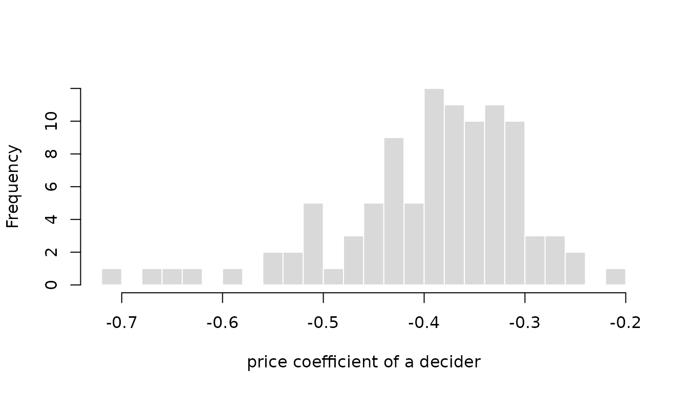
A picture says it faster. The histogram shows the price coefficient of each of the 400 deciders, with the three quantiles above marked. Every decider sits on the negative side, which is what the log-normal specification enforces, and the tail to the left holds those who react most strongly to a higher price.

price <- -exp(individual[, "price"])
hist(
  price,
  breaks = 30, col = "grey85", border = "white",
  main = "", xlab = "price coefficient of a decider"
)
abline(v = quantile(price, c(0.1, 0.5, 0.9)), lwd = 2)

How much is a local electricity supplier worth?

The Electricity data of the mlogit package (Croissant 2020) come from a stated choice experiment in which 361 US households chose 8 to 12 times among four hypothetical suppliers that differ in price (pf), contract length (cl), whether the supplier is local (loc) or well-known (wk), and whether it offers time-of-day (tod) or seasonal (seas) rates (Huber and Train 2001). Huber and Train (2001) used these data to check whether hierarchical Bayesian and classical estimates of individual preferences agree, and found that they largely do. The attribute columns end in the supplier number without a delimiter, pf1 to pf4, so an underscore is inserted first, and the choice occasions of a household are numbered in the order of the rows.

Contract length and locality receive correlated normal random coefficients, the other three attributes one coefficient for everyone. Keeping the number of random coefficients small is deliberate: each one adds a row and a column to every covariance draw, and the chains below have to be long enough that the result can be believed rather than merely displayed. Fixing the price coefficient to -1 identifies the scale and puts every other coefficient in cents per kWh, that is, expresses it directly as a willingness to pay. All six attributes have to enter the model: suppliers with time-of-day or seasonal rates carry a price of zero in these data, so leaving their dummies out would hand their missing price level to the price coefficient and turn it positive.

data("Electricity", package = "mlogit")
names(Electricity) <- sub("([a-z]+)([1-4])$", "\\1_\\2", names(Electricity))
Electricity$occasion <- ave(Electricity$id, Electricity$id, FUN = seq_along)
electricity <- fit(
  choice ~ pf + cl + loc + wk + tod + seas | 0,
  data = Electricity,
  random_effects = c("cl", "loc"),
  column_decider = "id",
  column_occasion = "occasion",
  scale = c(pf = -1),
  iterations = 3000,
  warmup = 1500,
  thin = 2,
  chains = 2,
  save_individual_draws = TRUE,
  progress = FALSE
)
summary(electricity)
#> Bayesian probit choice model
#> Formula: choice ~ pf + cl + loc + wk + tod + seas | 0 | 0 
#> Samples: 750 retained per chain, 2 chains
#> 
#>        variable    mean    mode     sd rhat ess_bulk
#>        beta[wk]  1.5224  1.5259 0.0754 1.01    295.9
#>       beta[tod] -8.7348 -8.7287 0.0765 1.01    200.5
#>      beta[seas] -9.2978 -9.2676 0.0840 1.02    216.6
#>          mu[cl] -0.2165 -0.2152 0.0274 1.01    723.4
#>         mu[loc]  2.0493  2.0366 0.1259 1.00    372.2
#>    Omega[cl,cl]  0.1886  0.1839 0.0223 1.00    359.5
#>   Omega[cl,loc]  0.0459  0.0402 0.0508 1.00    295.8
#>  Omega[loc,loc]  2.2652  2.1807 0.3320 1.00    326.6
#>      Sigma[2,2]  7.0883  7.0644 0.7139 1.03     52.8
#>      Sigma[2,3]  2.8021  2.6859 0.5159 1.04     43.3
#>      Sigma[3,3]  5.8244  5.7776 0.6674 1.00     99.8
#>      Sigma[2,4]  3.3193  3.1529 0.4972 1.12     18.0
#>      Sigma[3,4]  2.7979  2.6260 0.4605 1.03     59.3
#>      Sigma[4,4]  6.5651  6.3676 0.7563 1.11     16.1

The four supplier attributes other than price and contract length are dummy variables. Households dislike long contracts and prefer local and well-known suppliers, the three signs that the original analysis reports as well. Because the price coefficient is fixed, interpret() reads the means directly as willingness to pay in cents per kWh and attaches credible intervals:

interpret(electricity, effects = c("cl", "loc", "wk"))
#> 1 `cl` compensates -0.217 `pf` (95% interval -0.271 to -0.164)
#> 1 `loc` compensates 2.05 `pf` (95% interval 1.81 to 2.3)
#> 1 `wk` compensates 1.52 `pf` (95% interval 1.38 to 1.67)

On average, households would accept a price about 2 cents per kWh higher for a local supplier, and every additional year of contract length would have to be compensated by a price about 0.22 cents lower. The Omega[...] variables describe how widely these valuations differ between households: the standard deviation of the locality premium is 1.5 cents, so the households disagree about it by more than its average size.

A word on cost. This fit takes a few seconds because it draws one coefficient pair per household in every iteration. Doubling the households roughly doubles the time, and each further random coefficient adds a row and a column to every covariance draw. The five-attribute model on all 361 households that the original study used is a matter of minutes rather than seconds, and it needs far more than four thousand iterations before its covariance entries settle down.

Latent classes

A single normal distribution is a strong assumption about how preferences are spread across a population. Perhaps there are commuters and leisure travelers, or households that care about price and households that care about service. latent_class_effects names the effects that differ between classes latent classes. For a random effect this replaces its normal distribution by a finite mixture of normals, which yields the latent-class mixed multinomial probit model of Oelschläger and Bauer (2021); Oelschläger (2026b) places it among the broader challenges of modeling choice-behavior heterogeneity. Random effects that are not named keep one distribution for all deciders, and a named coefficient that is not random gets one value per class without varying within it, which a later subsection shows. Three different questions call for three different specifications:

class_update = "fixed" when exactly $K$ substantively meaningful classes are assumed;
class_update = "sparse" when classes is a deliberately generous upper bound and redundant classes should empty out;
class_update = "dirichlet_process" for a Dirichlet-process mixture whose number of occupied classes is itself random.

These models answer different questions, so pick one when you design the study rather than after seeing the class-specific results. A fourth option, class_update = "weight_based", reproduces the split/remove/merge heuristic of earlier RprobitB versions; it is a search procedure, not another Bayesian model.

All four updates are demonstrated on one simulated data set with two classes. The fixed-class fit simulates it; the other three are refits of it through update(), which reuses its simulated data and replaces only the arguments that are named, so that all updates are judged on identical observations. The empirical application is shown for the fixed update.

A fixed number of classes

For class_update = "fixed", classes = K fixes the number of classes and every class stays occupied, which is the direct specification for a filled $K$ -class model chosen a priori. If classes should instead be allowed to empty, that is the question the sparse finite mixture below answers.

The fixed model uses $(w_1,\ldots,w_K)\sim\operatorname{Dirichlet}(\delta,\ldots,\delta)$ . Its default class_concentration = 1 is uniform on the weight simplex; $\delta < 1$ favors unequal weights near its boundary and $\delta > 1$ shrinks weights toward $1/K$ . This prior remains influential when the likelihood separates the classes only weakly. It can be fixed to another positive scalar or given a gamma hyperprior with, for example, prior = list(class_concentration = c(shape = 2, rate = 2)). Report the choice and check sensitivity whenever class sizes drive the interpretation.

Which class is called the first one is arbitrary: swapping the labels leaves the likelihood unchanged, so the sampler may swap them mid-run and a posterior mean would average over both meanings. Ordering the classes by one parameter, say by decreasing weight, does not reliably repair this (Stephens 2000). RprobitB instead leaves the sampler free and relabels the retained draws afterwards. It reads off a representative grouping of the deciders from the posterior co-clustering matrix (Dahl 2006), matches every draw’s allocation to it (Papastamoulis and Iliopoulos 2010), and permutes weights, means, covariances, and allocations accordingly. Sorting the relabeled weights at the end is a naming convention, not the thing that identifies the classes.

The proof of concept uses eight occasions per decider and two well-separated classes: a majority whose coefficient is centered at -1 and a minority centered at 2. These conditions are deliberately favorable, because class-specific distributions are hard to learn from short panels. Two chains of four thousand iterations are long enough here that the diagnostics in the summary can be taken at face value.

mixture <- fit(
  choice ~ x | 0,
  random_effects = "x",
  latent_class_effects = "x",
  classes = 2,
  n_deciders = 80,
  n_occasions = 8,
  save_individual_draws = TRUE,
  dgp_parameters = list(
    beta = list(c(x = -1), c(x = 2)),
    Omega = list(matrix(0.2), matrix(0.2)),
    weights = c(0.6, 0.4)
  ),
  iterations = 4000,
  warmup = 2000,
  chains = 2,
  progress = FALSE
)
summary(mixture, variables = c(
  "weight[1]", "weight[2]", "mu[x,1]", "mu[x,2]",
  "Omega[x,x,1]", "Omega[x,x,2]"
))
#> Bayesian probit choice model
#> Formula: choice ~ x | 0 | 0 
#> Samples: 2000 retained per chain, 2 chains
#> 
#>      variable  dgp   mean   mode     sd rhat ess_bulk
#>     weight[1]  0.6  0.607  0.618 0.0601 1.00    398.3
#>     weight[2]  0.4  0.393  0.382 0.0601 1.00    398.3
#>       mu[x,1] -1.0 -0.761 -0.736 0.1087 1.00    335.4
#>       mu[x,2]  2.0  2.219  2.221 0.3363 1.03     56.1
#>  Omega[x,x,1]  0.2  0.201  0.141 0.0982 1.01    156.1
#>  Omega[x,x,2]  0.2  0.410  0.190 0.4110 1.01     46.7

The relabeled weights and means can be read class by class. The class near -1 holds about half of these 80 deciders, a little less than its population weight of 0.6, and the class near 2 the rest. The class variances are the least precise entries, but rhat stays at the threshold and the effective sample sizes are in the hundreds, so the table describes the posterior rather than one chain’s wanderings. That check is worth repeating for every mixture fit, because relabeling cannot repair poor mixing or weak class separation.

The three updates below relabel their draws in the same way, so their summaries carry class-specific weights and means as well. Where the number of classes varies, a class exists only in part of the draws, and the occupied column reports that share. Classes that no decider ever occupies are left out, which is why the class indices in the tables below may skip a number. The refits on shared data have no dgp column, so a small helper compares them with the stored truth: the most probable number of occupied classes, and, after assigning every decider to the true class whose mean is closer to their posterior mean coefficient, the share of deciders in the second class and the average coefficient in each class. The true weight is the population weight; the realized share among 80 simulated deciders differs from it by sampling variation.

truth <- mixture$simulation$dgp_parameters
class_means <- c(truth$beta[[1]][["x"]], truth$beta[[2]][["x"]])
recover_classes <- function(x) {
  occupancy <- latent_class_diagnostics(x)$occupancy
  individual <- coef(x, level = "individual")[, "x"]
  upper <- individual > mean(class_means)
  data.frame(
    variable = c("n_classes", "weight[2]", "mu[x,1]", "mu[x,2]"),
    dgp = c(length(truth$weights), truth$weights[2], class_means),
    estimate = c(
      occupancy$n_classes[which.max(occupancy$probability)],
      mean(upper), mean(individual[!upper]), mean(individual[upper])
    )
  )
}
recover_classes(mixture)
#>    variable  dgp   estimate
#> 1 n_classes  2.0  2.0000000
#> 2 weight[2]  0.4  0.4000000
#> 3   mu[x,1] -1.0 -0.7740019
#> 4   mu[x,2]  2.0  2.1637702

The two classes are visible in the individual coefficients. Each decider contributes one value, and the two estimated class means mark where the mixture places its classes.

individual_x <- coef(mixture, level = "individual")[, "x"]
hist(
  individual_x,
  breaks = 30, col = "grey85", border = "white",
  main = "", xlab = "x coefficient of a decider"
)
abline(v = coef(mixture)[c("mu[x,1]", "mu[x,2]")], lwd = 2)

Two clearly separated groups of deciders, one on either side of zero, and almost nobody in between: that is the pattern a mixture is meant to find. A single normal distribution would have to put most of its mass where no decider actually is.

The label-invariant co-clustering matrix and the allocation uncertainty are available regardless of class names:

class_diagnostics <- latent_class_diagnostics(mixture)
class_diagnostics$occupancy
#>   n_classes probability
#> 1         2           1
class_diagnostics$membership[1:6, ]
#>   class_1 class_2
#> 1 0.99500 0.00500
#> 2 0.99750 0.00250
#> 3 0.99625 0.00375
#> 4 0.99350 0.00650
#> 5 0.00025 0.99975
#> 6 0.99700 0.00300
class_diagnostics$co_clustering[1:6, 1:6]
#>         1       2       3       4       5       6
#> 1 1.00000 0.99400 0.99275 0.99050 0.00525 0.99250
#> 2 0.99400 1.00000 0.99425 0.99250 0.00275 0.99500
#> 3 0.99275 0.99425 1.00000 0.99125 0.00400 0.99425
#> 4 0.99050 0.99250 0.99125 1.00000 0.00675 0.99100
#> 5 0.00525 0.00275 0.00400 0.00675 1.00000 0.00325
#> 6 0.99250 0.99500 0.99425 0.99100 0.00325 1.00000

Asking for two filled classes is not evidence that two meaningful populations exist. When $K$ is not fixed by the research design, fit each candidate value to the same data and compare the decider-level predictive accuracy. The loo package (Vehtari et al. 2026) supplies the comparison and WAIC() is the less diagnostic alternative; vignette("v05_model_evaluation") covers both. Standard AIC() and BIC() also work, because logLik() returns a proper logLik object, but their asymptotic justification is fragile for mixtures, so PSIS-LOO is preferred.

models_by_K <- lapply(1:3, function(K) {
  class_effects <- if (K > 1) "x" else character()
  update(
    mixture, classes = K, latent_class_effects = class_effects,
    iterations = 2000, warmup = 1000, thin = 20
  )
})
loo::loo_compare(
  lapply(models_by_K, loo, ghk_draws = 50, progress = FALSE)
)
#> Warning: Some Pareto k diagnostic values are too high. See help('pareto-k-diagnostic') for details.
#> Warning: Some Pareto k diagnostic values are too high. See help('pareto-k-diagnostic') for details.
#> Warning: Some Pareto k diagnostic values are too high. See help('pareto-k-diagnostic') for details.
#>   model elpd_diff se_diff p_worse diag_diff      diag_elpd
#>  model2       0.0     0.0      NA           1 k_psis > 0.5
#>  model3      -0.5     0.5    0.88   N < 100 1 k_psis > 0.5
#>  model1     -11.3     3.5    1.00   N < 100 3 k_psis > 0.5
#> 
#> Diagnostic flags present.
#> See ?`loo-glossary` (sections `diag_diff` and `diag_elpd`)
#> or https://mc-stan.org/loo/reference/loo-glossary.html.

The two-class model wins over the one-class model by several standard errors, and the third class buys nothing: its expected predictive accuracy is within noise of the second. That is the answer one hopes for from data that were generated with two classes. The three fits are thinned and use fewer GHK draws than the default, because each loo() call evaluates the panel likelihood of every decider under every retained draw.

An empirical application of the fixed update follows in the next subsection, where the train travelers of vignette("v01_get_started") split into two classes with different values of time.

Coefficients that differ only between classes

The mixture above lets the coefficient vary within a class as well: every decider has their own x coefficient, drawn from the normal distribution of their class. The classical latent class model is stricter. All members of a class share the same coefficient, so the heterogeneity lives entirely in the class membership (Kamakura and Russell 1989; Greene and Hensher 2003), which market research knows as segmentation.

RprobitB fits this model when a covariate in latent_class_effects has no random effect: its fixed coefficient then takes one value per class, reported as beta[<effect>,<class>]. Random and class-specific effects share the class allocation, so a model may have classes that differ in their price coefficient while the time coefficient varies normally within each class, either with the same distribution in every class or, if time is named in both arguments, with class-specific distributions.

The proof of concept simulates two classes of travelers, a majority with a price coefficient of -2 and a minority with -0.5, who value time equally.

class_specific <- fit(
  choice ~ price + time | 0,
  latent_class_effects = "price",
  classes = 2,
  n_deciders = 300,
  n_occasions = 10,
  dgp_parameters = list(
    beta = list(c(price = -2, time = 1), c(price = -0.5, time = 1)),
    weights = c(0.6, 0.4)
  ),
  chains = 1
)
summary(class_specific)
#> Bayesian probit choice model
#> Formula: choice ~ price + time | 0 | 0 
#> Samples: 500 retained per chain, 1 chain
#>       variable  dgp   mean   mode     sd rhat ess_bulk
#>     beta[time]  1.0  0.972  0.978 0.0365 1.02    28.49
#>      weight[1]  0.6  0.615  0.614 0.0364 1.04    85.30
#>      weight[2]  0.4  0.385  0.386 0.0364 1.04    85.30
#>  beta[price,1] -2.0 -2.035 -2.065 0.0947 1.24     4.27
#>  beta[price,2] -0.5 -0.455 -0.453 0.0454 1.15     6.96

The estimated class weights of 0.61 and 0.39 and the class-specific price coefficients of -2.03 and -0.46 are close to the values used for the simulation, and the common time coefficient is estimated from all deciders at once. Since every class has its own price coefficient, interpret() reports one willingness to pay per class:

interpret(class_specific, reference = "price")
#> Class 1: 1 `time` compensates 0.478 `price` (95% interval 0.443 to 0.522)
#> Class 2: 1 `time` compensates 2.16 `price` (95% interval 1.74 to 2.65)

Back to the train travelers of vignette("v01_get_started"): do all of them trade time against money at the same rate, or are there classes with different values of time? The fit below uses the first 100 travelers, keeps the price normalization, and gives the time coefficient two class-specific values, so that each class has its own value of an hour of travel time, while the remaining coefficients are common.

data("Train", package = "mlogit")
Train$price_A <- Train$price_A / 100 / 2.20371
Train$price_B <- Train$price_B / 100 / 2.20371
Train$time_A <- Train$time_A / 60
Train$time_B <- Train$time_B / 60
train_small <- Train[Train$id %in% unique(Train$id)[1:100], ]
train_classes <- fit(
  choice ~ price + time + change + factor(comfort) | 0,
  data = train_small,
  latent_class_effects = "time",
  classes = 2,
  column_decider = "id",
  column_occasion = "choiceid",
  scale = c(price = -1),
  iterations = 2500,
  warmup = 1250,
  chains = 2,
  progress = FALSE
)
summary(train_classes, variables = c(
  "weight[1]", "weight[2]", "beta[time,1]", "beta[time,2]"
))
#> Bayesian probit choice model
#> Formula: choice ~ price + time + change + factor(comfort) | 0 | 0 
#> Samples: 1250 retained per chain, 2 chains
#> 
#>      variable    mean    mode     sd rhat ess_bulk
#>     weight[1]   0.862   0.882 0.0577 1.01     86.4
#>     weight[2]   0.138   0.118 0.0577 1.01     86.4
#>  beta[time,1]  -3.465  -3.536 0.6788 1.02    113.7
#>  beta[time,2] -20.444 -19.017 5.3399 1.04     52.1

With the price coefficient fixed at -1, the class-specific time coefficients are values of travel time in euro per hour, which interpret() reports class by class:

time_by_class <- interpret(train_classes, effects = "time")
time_by_class
#> Class 1: 1 `time` compensates -3.47 `price` (95% interval -4.74 to -2.15)
#> Class 2: 1 `time` compensates -20.4 `price` (95% interval -36.1 to -13.2)

The larger class of 86 percent of the travelers values an hour at 3.5 euro, the smaller class at 20.4 euro. The small class takes the faster trip almost regardless of its price, a pattern that a single normal distribution of the time coefficient would blur into a heavy tail. The diagnostics of both weights and both time coefficients are sound, so this is a result rather than a demonstration.

Weight-based class updates

The weight-based update of Oelschläger and Bauer (2021) is kept for backward compatibility and for reproducing earlier RprobitB analyses; Oelschläger (2026b) discusses its broader context. Every buffer warmup iterations, the heuristic attempts at most one operation, in this order:

remove the smallest class if its weight is below epsmin;
split the largest class if its weight is above epsmax;
merge the closest pair if the Euclidean distance of their means is below deltamin.

After a split, the new means are displaced by deltashift times the leading within-class standard deviation. The original defaults are buffer = 50, epsmin = 0.01, epsmax = 0.7, deltamin = 0.1, and deltashift = 0.5; override them with weight_based_control. max_classes bounds the splitting.

These dimension changes have no Metropolis-Hastings acceptance step and correspond to no prior on the class count. Updates stop after warmup, so the retained draws condition on whatever dimension each chain selected. The reported n_classes is accordingly a heuristic result, not a posterior distribution. There is no universally valid calibration of the five constants: any use should report them and repeat the analysis over substantively plausible settings. For inferential claims, prefer the fixed, sparse finite, or Dirichlet-process specifications.

The proof of concept keeps the update defaults, and a second run tightens two of the five constants through weight_based_control: it checks more often and refuses to split a class before its weight passes 0.8.

weight_based <- update(mixture, class_update = "weight_based")
recover_classes(weight_based)
#>    variable  dgp   estimate
#> 1 n_classes  2.0  2.0000000
#> 2 weight[2]  0.4  0.4000000
#> 3   mu[x,1] -1.0 -0.7775812
#> 4   mu[x,2]  2.0  2.0861235
tuned <- update(
  mixture,
  class_update = "weight_based",
  weight_based_control = list(buffer = 25, epsmax = 0.8)
)
recover_classes(tuned)
#>    variable  dgp  estimate
#> 1 n_classes  2.0  2.000000
#> 2 weight[2]  0.4  0.400000
#> 3   mu[x,1] -1.0 -0.769339
#> 4   mu[x,2]  2.0  2.167189

The heuristic keeps both classes, and the share and the class means come out as in the table of the fixed fit. That is what it was designed for; the caveats above concern what its result means, not whether it can find two well-separated classes.

Sparse finite mixtures

A sparse finite mixture fixes a generous upper bound $K$ , permits empty classes, and places a symmetric Dirichlet prior

$(w_1,\ldots,w_K) \mid e_0 \sim \operatorname{Dirichlet}(e_0,\ldots,e_0)$

on the weights. A small $e_0$ favors emptying redundant classes. Under regularity conditions, overfitted classes empty asymptotically when the Dirichlet parameter is below half the dimension of a class-specific parameter (Rousseau and Mengersen 2011). This result motivates sparsity but does not make the prior harmless: both $K$ and $e_0$ affect the posterior of the occupied count (Frühwirth-Schnatter and Malsiner-Walli 2019).

Before looking at the data, the expected number of occupied classes after $N$ deciders under a fixed $e_0$ is

$K\left[1- \frac{\Gamma(Ke_0)\,\Gamma((K-1)e_0+N)} {\Gamma((K-1)e_0)\,\Gamma(Ke_0+N)}\right].$

The expression makes $e_0$ readable as a statement about class counts instead of an arbitrary small number. Evaluated at the prior mean $e_0 = 0.005$ of the default hyperprior below, with $K = 6$ and the 80 deciders of the simulated data, it gives about 1.1 occupied classes: the prior leans firmly towards simplicity. For a gamma hyperprior, draw plausible values of $e_0$ , evaluate the expression, and inspect the implied distribution before fitting.

Unlike the threshold-based updater, class_update = "sparse" uses the finite-mixture posterior itself to empty classes. The default class_concentration = c(shape = 1, rate = 200) puts the gamma hyperprior $e_0\sim\operatorname{Gamma}(1,200)$ on the shape-rate scale used by R. The concentration is updated from its full conditional with a fixed log-random-walk Metropolis-Hastings step. Its proposal scale affects the sampling efficiency, not the posterior target; rhat and the effective sample size diagnose that step like any other scalar posterior variable.

The proof of concept offers six classes to the two-class data.

sparse <- update(mixture, classes = 6, class_update = "sparse")
summary(sparse)
#> Bayesian probit choice model
#> Formula: choice ~ x | 0 | 0 
#> Samples: 2000 retained per chain, 2 chains
#> 
#>             variable occupied    mean     mode      sd rhat ess_bulk
#>            weight[1]   1.0000  0.6052  0.60309 0.06094 1.02   153.05
#>            weight[2]   1.0000  0.3897  0.39594 0.06006 1.01   463.12
#>            weight[3]   0.0777  0.0293  0.01278 0.02906   NA       NA
#>            weight[4]   0.0437  0.0229  0.00876 0.02191   NA       NA
#>            weight[5]   0.0385  0.0251  0.00825 0.02953   NA       NA
#>            weight[6]   0.0135  0.0238  0.00673 0.02227   NA       NA
#>              mu[x,1]   1.0000 -0.7565 -0.75269 0.11194 1.01   320.44
#>              mu[x,2]   1.0000  2.1569  2.05099 0.31389 1.01    85.14
#>              mu[x,3]   0.0777 -3.3113 -4.99881 3.27128   NA       NA
#>              mu[x,4]   0.0437 -4.5646 -5.92321 2.85016   NA       NA
#>              mu[x,5]   0.0385 -2.4835 -4.92683 2.74781   NA       NA
#>              mu[x,6]   0.0135  0.5556  1.49981 1.82207   NA       NA
#>         Omega[x,x,1]   1.0000  0.2038  0.15520 0.12780 1.01   113.73
#>         Omega[x,x,2]   1.0000  0.4386  0.19973 0.42241 1.05    41.13
#>         Omega[x,x,3]   0.0777  1.2866  0.27913 2.86642   NA       NA
#>         Omega[x,x,4]   0.0437  2.3528  0.36528 4.62401   NA       NA
#>         Omega[x,x,5]   0.0385  0.6045  0.26114 0.60467   NA       NA
#>         Omega[x,x,6]   0.0135  0.4845  0.33944 0.41081   NA       NA
#>  class_concentration   1.0000  0.0104  0.00536 0.00623 1.03    85.69
#>            n_classes   1.0000  2.1735  2.00000 0.42361 1.26     6.49
latent_class_diagnostics(sparse)$occupancy
#>   n_classes probability
#> 1         2      0.8440
#> 2         3      0.1390
#> 3         4      0.0165
#> 4         5      0.0005
recover_classes(sparse)
#>    variable  dgp   estimate
#> 1 n_classes  2.0  2.0000000
#> 2 weight[2]  0.4  0.4000000
#> 3   mu[x,1] -1.0 -0.7905144
#> 4   mu[x,2]  2.0  2.1060220

Despite the prior’s preference for a single class, the occupied count concentrates on two, and the class structure is recovered as by the fixed model. The concentration parameter is the slowest-mixing quantity, as its effective sample size shows. A sensitivity analysis should be run with longer chains until both n_classes and class_concentration mix satisfactorily.

For a sensitivity analysis, vary the upper bound and the concentration prior, then compare occupancy, co-clustering, predictive accuracy, and the substantive conclusions. A useful less-sparse alternative is $e_0\sim\operatorname{Gamma}(2,4K)$ , whose expected total mass $K e_0$ matches the default DP precision below (Frühwirth-Schnatter and Malsiner-Walli 2019).

sparse_less <- update(
  mixture,
  classes = 6,
  class_update = "sparse",
  prior = list(class_concentration = c(shape = 2, rate = 24))
)
latent_class_diagnostics(sparse_less)$occupancy
#>   n_classes probability
#> 1         2     0.41825
#> 2         3     0.35425
#> 3         4     0.17250
#> 4         5     0.05000
#> 5         6     0.00500
recover_classes(sparse_less)
#>    variable  dgp   estimate
#> 1 n_classes  2.0  2.0000000
#> 2 weight[2]  0.4  0.4000000
#> 3   mu[x,1] -1.0 -0.7746666
#> 4   mu[x,2]  2.0  2.2480394

Six classes on offer and a prior that resists emptying them: the occupied count now spreads from two to five instead of concentrating on two. The class means are still recovered, because the extra classes hold few deciders, but the answer to the question how many classes there are has changed with the prior. That is exactly what a sensitivity analysis is for, and it is the reason to report the concentration prior alongside the occupancy table rather than the table alone.

Dirichlet-process mixtures

For class_update = "dirichlet_process", the precision $\alpha$ controls the prior tendency to open new classes. The default $\alpha\sim\operatorname{Gamma}(2,4)$ has mean 0.5; a larger $\alpha$ generally favors more occupied classes. Conditional on a fixed $\alpha$ , the Chinese-restaurant-process prior expects $\sum_{i=1}^{N}\alpha/(\alpha+i-1)$ occupied classes after $N$ deciders, which for $\alpha = 0.5$ and 80 deciders is about 3.2. Use this quantity to translate beliefs about plausible class counts into candidate values or gamma hyperpriors. RprobitB updates $\alpha$ with the beta-gamma augmentation of Escobar and West (1995) and the allocations with the auxiliary-parameter algorithm of Neal (2000), using ten auxiliary classes per reassignment; this choice affects computation and mixing, not the posterior target. max_classes is a computational cap, not the inferred count: if posterior mass reaches the cap, refit with a larger value.

The proof of concept lets the process decide how many classes the two-class data need.

dynamic <- update(
  mixture, class_update = "dirichlet_process", iterations = 2500,
  warmup = 1250
)
#> Warning: The retained draws reach the maximum of 10 latent classes.
#> ℹ Increase `max_classes` and refit to check the bound.
summary(dynamic)
#> Bayesian probit choice model
#> Formula: choice ~ x | 0 | 0 
#> Samples: 1250 retained per chain, 2 chains
#> 
#>             variable occupied    mean    mode      sd rhat ess_bulk
#>            weight[1]   1.0000  0.5755  0.5998 0.06900 1.08     89.6
#>            weight[2]   1.0000  0.3426  0.3936 0.06616 1.08     22.4
#>            weight[3]   0.6664  0.0859  0.0211 0.06990   NA       NA
#>            weight[4]   0.3452  0.0486  0.0152 0.04889   NA       NA
#>            weight[5]   0.1468  0.0386  0.0130 0.04354   NA       NA
#>            weight[6]   0.0596  0.0303  0.0133 0.02723   NA       NA
#>            weight[7]   0.0180  0.0194  0.0126 0.00981   NA       NA
#>            weight[8]   0.0060  0.0158  0.0125 0.00742   NA       NA
#>            weight[9]   0.0008  0.0125  0.0125 0.00000   NA       NA
#>           weight[10]   0.0004  0.0125  0.0125      NA   NA       NA
#>              mu[x,1]   1.0000 -0.7774 -0.7718 0.12929 1.01    218.1
#>              mu[x,2]   1.0000  2.2453  2.0450 0.48657 1.05     19.8
#>              mu[x,3]   0.6664  1.3931  1.9046 2.03380   NA       NA
#>              mu[x,4]   0.3452  0.9453 -0.3744 2.00520   NA       NA
#>              mu[x,5]   0.1468  1.3063 -0.4964 2.19466   NA       NA
#>              mu[x,6]   0.0596  0.9675  1.0852 1.96649   NA       NA
#>              mu[x,7]   0.0180  1.4371  1.8935 2.33256   NA       NA
#>              mu[x,8]   0.0060  1.3424  0.5347 2.34234   NA       NA
#>              mu[x,9]   0.0008  0.1415 -0.4154 0.79075   NA       NA
#>             mu[x,10]   0.0004 -2.5077 -2.5077      NA   NA       NA
#>         Omega[x,x,1]   1.0000  0.1916  0.1377 0.10038 1.03     86.4
#>         Omega[x,x,2]   1.0000  0.4715  0.1846 0.60096 1.04     85.2
#>         Omega[x,x,3]   0.6664  0.6610  0.2078 0.96489   NA       NA
#>         Omega[x,x,4]   0.3452  0.7436  0.2636 1.10819   NA       NA
#>         Omega[x,x,5]   0.1468  0.8780  0.2897 1.30039   NA       NA
#>         Omega[x,x,6]   0.0596  1.0189  0.2729 2.22782   NA       NA
#>         Omega[x,x,7]   0.0180  1.0172  0.4340 1.21229   NA       NA
#>         Omega[x,x,8]   0.0060  0.9291  0.2962 1.19804   NA       NA
#>         Omega[x,x,9]   0.0008  0.1284  0.1726 0.06282   NA       NA
#>        Omega[x,x,10]   0.0004  0.5693  0.5693      NA   NA       NA
#>  class_concentration   1.0000  0.5097  0.3384 0.29316 1.01    276.8
#>            n_classes   1.0000  3.2432  2.0000 1.24606 1.03     46.2
latent_class_diagnostics(dynamic)$occupancy
#>   n_classes probability
#> 1         2      0.3336
#> 2         3      0.3212
#> 3         4      0.1984
#> 4         5      0.0872
#> 5         6      0.0416
#> 6         7      0.0120
#> 7         8      0.0052
#> 8         9      0.0004
#> 9        10      0.0004
recover_classes(dynamic)
#>    variable  dgp   estimate
#> 1 n_classes  2.0  2.0000000
#> 2 weight[2]  0.4  0.4000000
#> 3   mu[x,1] -1.0 -0.7829333
#> 4   mu[x,2]  2.0  2.2380596

max_classes caps how many classes the sampler may open. The cap is a computational limit, not an estimate, and RprobitB says so when the draws reach it:

capped <- update(dynamic, max_classes = 3)
#> Warning: The retained draws reach the maximum of 3 latent classes.
#> ℹ Increase `max_classes` and refit to check the bound.
latent_class_diagnostics(capped)$occupancy
#>   n_classes probability
#> 1         2       0.518
#> 2         3       0.482

The warning is the signal to refit with a larger cap before reading the occupancy table.

The occupancy distribution is wider than under the sparse finite prior and keeps a substantial share of its mass on three or more classes. That is the prior at work: for a data set of this size it expects about three occupied classes, and 80 deciders do not overrule it completely. The label-invariant comparison nevertheless recovers the two true groups, because any superfluous class holds only a few deciders. Whether the occupancy table can be trusted is decided by the rhat and the effective sample size of the occupied count. Both are acceptable here, though the effective sample size of n_classes is the smallest in the table: enough for the broad shape of the distribution, not for its third decimal. The run stays below the cap, so the remaining step is a sensitivity analysis over the prior on $\alpha$ . Material mass at the cap would be a different matter: increase max_classes before interpreting the result.

The two priors can be compared directly by the posterior of the occupied count. The sparse finite prior concentrates on the two classes that the data contain, the Dirichlet process spreads its mass wider and keeps classes that hold only a few deciders.

occupancy_shares <- function(x, bound) {
  occupancy <- latent_class_diagnostics(x)$occupancy
  shares <- stats::setNames(numeric(bound), seq_len(bound))
  shares[occupancy$n_classes] <- occupancy$probability
  shares
}
bound <- max(
  latent_class_diagnostics(sparse)$occupancy$n_classes,
  latent_class_diagnostics(dynamic)$occupancy$n_classes
)
barplot(
  rbind(
    "sparse finite" = occupancy_shares(sparse, bound),
    "Dirichlet process" = occupancy_shares(dynamic, bound)
  ),
  beside = TRUE, col = c("grey60", "grey85"), border = "white",
  xlab = "occupied classes", ylab = "posterior probability", legend.text = TRUE,
  args.legend = list(x = "topright", bty = "n")
)

The occupied class count, the concentration, and the co-clustering probabilities do not refer to class labels at all and are therefore the safest summaries here. The relabeled class-specific parameters come with their occupied share: a class that exists in only a small fraction of the draws describes a handful of deciders, not a group in the population. Read the two together, and treat classes with a small share as sampling noise rather than as findings.

The prior on $\alpha$ belongs in the reported analysis. For example, $\alpha\sim\operatorname{Gamma}(1,200/K)$ has the same prior mean as $K e_0$ under the default sparse finite prior. Comparing this matched DP fit with a sparse finite fit helps separate the effect of the mixing model from that of the concentration prior (Frühwirth-Schnatter and Malsiner-Walli 2019). In every case, report the prior, the posterior of class_concentration, the occupancy distribution, whether the cap was reached, and the sensitivity to defensible alternatives.

Ordered and ranked responses

Both mechanisms work for ordered and ranked responses as well. What they need is a panel: a population distribution is learned from deciders observed repeatedly, and the ordered and ranked data sets of the previous vignettes record one response per decider. The demonstration therefore uses a simulated panel of rankings, 100 deciders who order three alternatives five times each, whose coefficient varies normally around -1.

ranked_random <- fit(
  rank ~ x | 0,
  choice_type = "ranked",
  random_effects = "x",
  n_deciders = 100,
  n_occasions = 5,
  n_alternatives = 3,
  dgp_parameters = list(beta = c(x = -1), Omega = matrix(0.3)),
  iterations = 4000,
  warmup = 2000,
  chains = 2,
  progress = FALSE
)
summary(ranked_random)
#> Bayesian probit choice model
#> Formula: rank ~ x | 0 | 0 
#> Samples: 2000 retained per chain, 2 chains
#> 
#>    variable   dgp   mean   mode     sd rhat ess_bulk
#>       mu[x] -1.00 -1.080 -1.070 0.0998 1.00      247
#>  Omega[x,x]  0.30  0.339  0.295 0.1029 1.01      184
#>  Sigma[B,C]  1.19  0.952  0.983 0.1827 1.00      443
#>  Sigma[C,C]  5.27  4.768  4.406 0.9124 1.00      317

The population mean and its variance are recovered next to their true values, and a full ranking of three alternatives per occasion carries enough information to do so from a hundred deciders. Latent classes are requested the same way, with latent_class_effects and classes, and everything this vignette says about relabeling, occupancy, and the concentration priors applies unchanged.

Ordered responses accept the same arguments. Here a hundred deciders rate something on a three-point scale eight times each, again with a coefficient that varies normally around -1.

ordered_random <- fit(
  choice ~ x | 0,
  alternatives = c("low", "middle", "high"),
  choice_type = "ordered",
  random_effects = "x",
  n_deciders = 100,
  n_occasions = 8,
  dgp_parameters = list(
    beta = c(x = -1), Omega = matrix(0.3), gamma = c(0, 1)
  ),
  iterations = 4000,
  warmup = 2000,
  chains = 2,
  progress = FALSE
)
summary(ordered_random)
#> Bayesian probit choice model
#> Formula: choice ~ x | 0 | 0 
#> Samples: 2000 retained per chain, 2 chains
#> 
#>    variable  dgp   mean   mode     sd rhat ess_bulk
#>       mu[x] -1.0 -1.060 -1.044 0.0956 1.01      320
#>  Omega[x,x]  0.3  0.363  0.319 0.1079 1.02      189
#>    gamma[2]  1.0  1.097  1.119 0.0597 1.01      404

The threshold gamma[2] is estimated alongside the population mean and its variance, and its diagnostics are worth a look: the thresholds are the one block of an ordered model that no Gibbs step can draw in closed form, so they are updated by a random walk whose step size is tuned during warmup. That tuning is what keeps the gamma rows mixing once random coefficients enter, and a long panel makes the thresholds easier still to pin down. Read their rhat and effective sample size the way vignette("v01_get_started") reads any diagnostic.

Where to go next

Heterogeneity pays off in prediction: with individual coefficients in hand, predict(type = "conditional") in vignette("v04_prediction") tailors the choice probabilities to each decider that took part in the fit. Deciding how many classes the data support, or whether random coefficients are worth their price at all, is the business of vignette("v05_model_evaluation").

References

Allenby, Greg M., and Peter E. Rossi. 1998. “Marketing Models of Consumer Heterogeneity.” Journal of Econometrics 89 (1-2): 57–78. https://doi.org/10.1016/S0304-4076(98)00055-4.

Croissant, Yves. 2020. “Estimation of Random Utility Models in R: The mlogit Package.” Journal of Statistical Software 95 (11): 1–41. https://doi.org/10.18637/jss.v095.i11.

Dahl, David B. 2006. “Model-Based Clustering for Expression Data via a Dirichlet Process Mixture Model.” In Bayesian Inference for Gene Expression and Proteomics, edited by Kim-Anh Do, Peter Müller, and Marina Vannucci. Cambridge University Press. https://doi.org/10.1017/CBO9780511584589.011.

Escobar, Michael D., and Mike West. 1995. “Bayesian Density Estimation and Inference Using Mixtures.” Journal of the American Statistical Association 90 (430): 577–88. https://doi.org/10.1080/01621459.1995.10476550.

Frühwirth-Schnatter, Sylvia, and Gertraud Malsiner-Walli. 2019. “From Here to Infinity: Sparse Finite Versus Dirichlet Process Mixtures in Model-Based Clustering.” Advances in Data Analysis and Classification 13 (1): 33–64. https://doi.org/10.1007/s11634-018-0329-y.

Greene, William H., and David A. Hensher. 2003. “A Latent Class Model for Discrete Choice Analysis: Contrasts with Mixed Logit.” Transportation Research Part B: Methodological 37 (8): 681–98. https://doi.org/10.1016/S0191-2615(02)00046-2.

Huber, Joel, and Kenneth Train. 2001. “On the Similarity of Classical and Bayesian Estimates of Individual Mean Partworths.” Marketing Letters 12 (3): 259–69. https://doi.org/10.1023/A:1011120928698.

Kamakura, Wagner A., and Gary J. Russell. 1989. “A Probabilistic Choice Model for Market Segmentation and Elasticity Structure.” Journal of Marketing Research 26 (4): 379–90.

Neal, Radford M. 2000. “Markov Chain Sampling Methods for Dirichlet Process Mixture Models.” Journal of Computational and Graphical Statistics 9 (2): 249–65. https://doi.org/10.1080/10618600.2000.10474879.

Oelschläger, Lennart. 2026a. choicedata: Working with Choice Data. https://github.com/loelschlaeger/choicedata.

Oelschläger, Lennart. 2026b. “Overcoming Challenges in Modeling Choice Behavior Heterogeneity.” PhD thesis, Bielefeld University. https://pub.uni-bielefeld.de/record/3014719.

Oelschläger, Lennart, and Dietmar Bauer. 2021. “Bayes Estimation of Latent Class Mixed Multinomial Probit Models.” Proceedings of the 100th Annual Meeting of the Transportation Research Board (Washington, DC). https://trid.trb.org/view/1759753.

Oelschläger, Lennart, and Dietmar Bauer. 2026. RprobitB: Bayesian Probit Choice Modeling. https://CRAN.R-project.org/package=RprobitB.

Papastamoulis, Panagiotis, and George Iliopoulos. 2010. “An Artificial Allocations Based Solution to the Label Switching Problem in Bayesian Analysis of Mixtures of Distributions.” Journal of Computational and Graphical Statistics 19 (2): 313–31. https://doi.org/10.1198/jcgs.2010.09008.

Rousseau, Judith, and Kerrie Mengersen. 2011. “Asymptotic Behaviour of the Posterior Distribution in Overfitted Mixture Models.” Journal of the Royal Statistical Society: Series B (Statistical Methodology) 73 (5): 689–710. https://doi.org/10.1111/j.1467-9868.2011.00781.x.

Stephens, Matthew. 2000. “Dealing with Label Switching in Mixture Models.” Journal of the Royal Statistical Society: Series B (Statistical Methodology) 62 (4): 795–809. https://doi.org/10.1111/1467-9868.00265.

Vehtari, Aki, Jonah Gabry, Måns Magnusson, et al. 2026. loo: Efficient Leave-One-Out Cross-Validation and WAIC for Bayesian Models. https://mc-stan.org/loo/.