Visualize fitted probit model

This function is the plot method for an object of class RprobitB_fit.

Usage

# S3 method for class 'RprobitB_fit'
plot(x, type, ignore = NULL, ...)

Arguments

x

An object of class RprobitB_fit.

type

[character(1)]
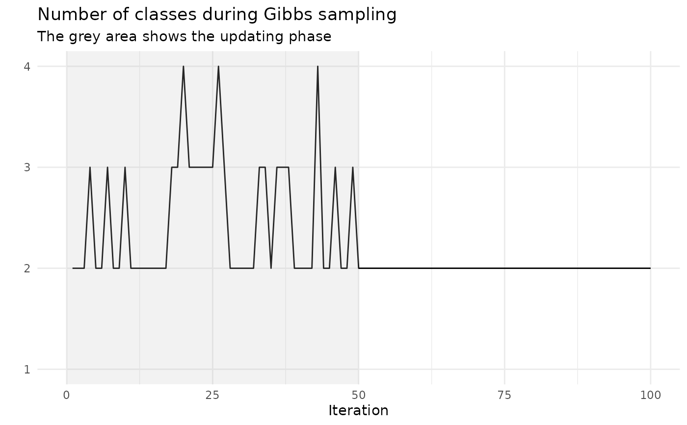
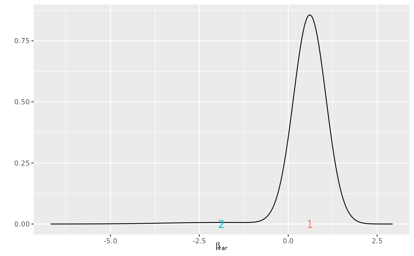
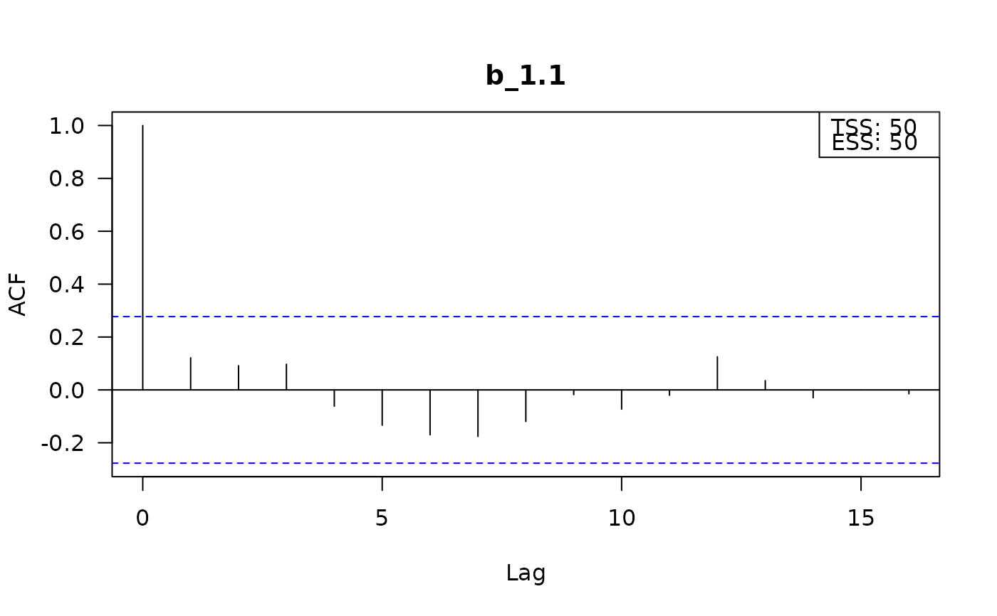
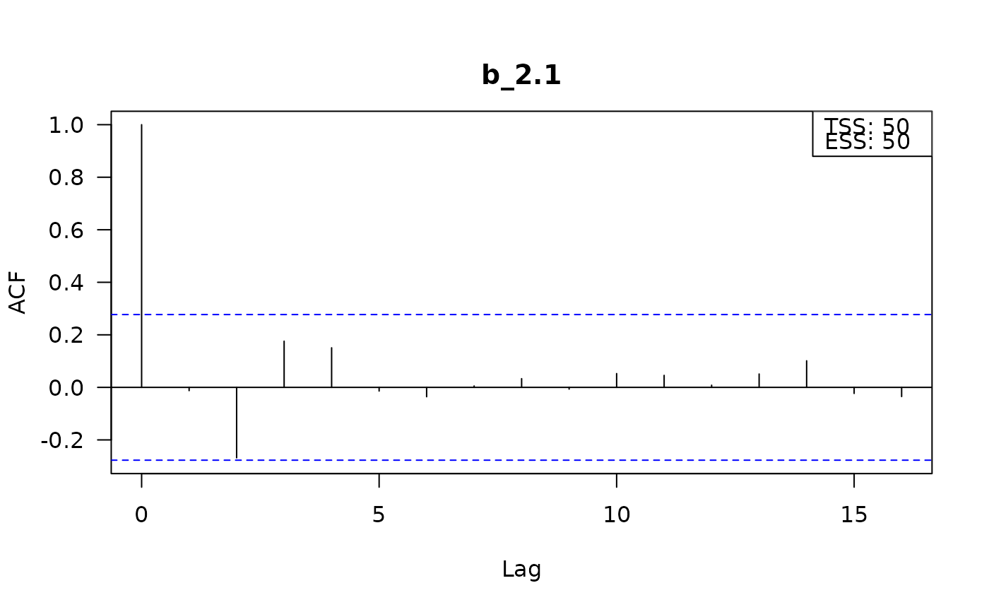
The type of plot, which can be one of:

• "mixture" to visualize the mixing distribution,

• "acf" for autocorrelation plots of the Gibbs samples,

• "trace" for trace plots of the Gibbs samples,

• "class_seq" to visualize the sequence of class numbers.

ignore

[character()]
Covariate or parameter names that do not get visualized.

...

Currently not used.

Value

No return value. Draws a plot to the current device.

Examples

set.seed(1)
form <- choice ~ var | 0
data <- simulate_choices(form = form, N = 100, T = 10, J = 3, re = "var")
model <- fit_model(
  data = data, R = 100, latent_classes = list(C = 2, "dp_update" = TRUE)
)
#> Computing sufficient statistics - 0 of 4  

#> Computing sufficient statistics - 1 of 4  

#> Computing sufficient statistics - 2 of 4  

#> Computing sufficient statistics - 3 of 4  

#> Computing sufficient statistics - 4 of 4  

#> Gibbs sampler - 1 of 100 iterations (C = 2) 

#> Gibbs sampler - 10 of 100 iterations (C = 2) 

#> Gibbs sampler - 20 of 100 iterations (C = 3) 

#> Gibbs sampler - 30 of 100 iterations (C = 2) 

#> Gibbs sampler - 40 of 100 iterations (C = 2) 

#> Gibbs sampler - 50 of 100 iterations (C = 3) 

#> Gibbs sampler - 60 of 100 iterations (C = 2) 

#> Gibbs sampler - 70 of 100 iterations (C = 2) 

#> Gibbs sampler - 80 of 100 iterations (C = 2) 

#> Gibbs sampler - 90 of 100 iterations (C = 2) 

#> Gibbs sampler - 100 of 100 iterations (C = 2) 

plot(model, type = "mixture")

plot(model, type = "acf", ignore = c("s", "Omega", "Sigma"))


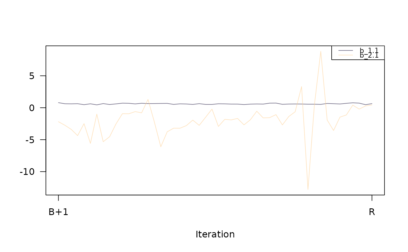
plot(model, type = "trace", ignore = c("s", "Omega", "Sigma"))

plot(model, type = "class_seq")